Introduction

A classic volume profile slices the chart into horizontal price levels and asks how much volume traded at each one. That works beautifully in a range and badly in a trend, for a reason that is obvious once you say it out loud: if price has climbed 15% over the window, the “high volume node” you get is mostly an artefact of how long price spent on its way up. The profile is measuring the trend, not the auction.

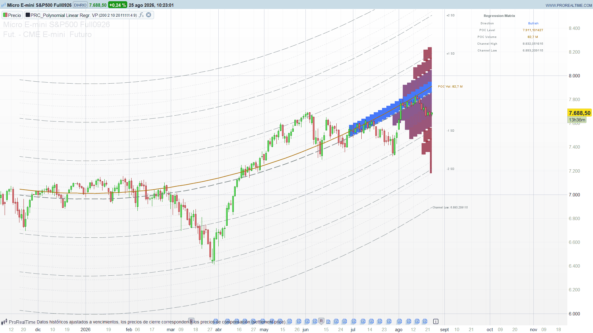
The Polynomial/Linear Regression Volume Profile by BigBeluga fixes that by changing the coordinate system. It first fits a regression curve — a straight line or a parabola — through the last N bars. Then it builds its price grid around that curve rather than around a fixed price, and assigns each bar’s volume to a row according to how far it closed from the curve, not according to its absolute price.

The result is a detrended volume profile. The Point of Control is no longer a horizontal level: it is a curve running parallel to the trend, marking the distance from the regression at which the market has done most of its business. When price is far from that curve, it is far from where the volume is, in a sense that stays meaningful whether the market is flat or up 20%.

Theory Behind the Indicator

1. The fit: least squares, straight or curved

The indicator fits y = b0 + b1·t + b2·t² to the source over the last regLen bars, by ordinary least squares. Set the degree to 1 and the quadratic term disappears, leaving a conventional regression channel. Set it to 2 and the curve is free to bend, which is the interesting case: a parabola captures a trend that is accelerating or, more usefully, one that is rolling over.

The abscissa is centred and normalised so that it runs from -1 at the oldest bar of the window to +1 at the most recent. That is not cosmetic. When the abscissa is symmetric about zero, the odd-power sums vanish — the sum of t is zero and so is the sum of t³ — and the normal equations collapse into four closed-form divisions:

b1  = sum(t·y) / sum(t²)
det = n·sum(t⁴) - sum(t²)²
b0  = (sum(y)·sum(t⁴) - sum(t²)·sum(t²·y)) / det
b2  = (n·sum(t²·y) - sum(t²)·sum(y)) / det

No matrix algebra, no inversion, and — because the condition number of the normal system drops from roughly 2.8e9 with raw powers of the bar index to 13.9 with the centred abscissa — no slow accumulation of rounding error either. Anyone who has tried to fit a cubic or a quartic on a long window knows exactly why that matters.

2. The grid: rows measured in standard deviations

Around the fitted curve the indicator draws numBins parallel levels on each side. The spacing is 3·SD / numBins, chosen so the outermost row lands exactly on ±3 SD. On top of that it draws the ±1, ±2 and ±3 SD curves themselves, which is where the channel gets its familiar shape.

Every row is a parallel copy of the regression curve, so the whole grid bends with the trend. A bar sitting “in the third row above the curve” means the same thing at the start of the window as at the end.

3. The profile: volume by distance from the curve

This is the core of the idea. For each bar in the window:

diff = source - fitted value at that bar
row  = floor(diff / rowHeight) + numBins

and the bar’s volume is added to that row. Once every bar has voted, each row is drawn as a horizontal bar that starts at the last candle and grows leftwards, with a length proportional to its share of the busiest row. The colour is interpolated from a muted red for the quiet rows to the trend colour — blue when the fit is rising, orange when it is falling — for the busy ones.

Note what the rows are not: they are not price levels. Row 12 is a band of distance from the regression, and on the chart it is drawn as a curve, not a horizontal line. Two bars that traded at completely different prices land in the same row if they were equally far above their respective fitted values.

4. The Point of Control

The row with the most volume is the POC, and it is extended across the whole window as a solid curve. This is the line worth watching. It is the level — in detrended terms — where the market has agreed the most, and price crossing it is a genuinely different event from price crossing a horizontal high-volume node, because it survives the trend being there.

The panel in the top right reports the direction of the fit, the current price of the POC curve, the volume that sits in that row, and the two channel extremes.

An Honest Look at the Standard Deviation

There is one design decision in this indicator that deserves to be flagged, because it changes what you see on the chart.

The standard deviation used to size the grid is the standard deviation of the source series, not of the residuals around the fitted curve. In a trending market those two numbers are very different: the first one is dominated by the excursion of the trend itself, the second measures actual dispersion around the fit. Since the row height is 3·SD / numBins, an inflated SD makes every row too tall, and the profile loses its resolution.

Measured on synthetic series of 200 bars with 20 rows, counting how many rows receive any volume at all:

• gently curving market — SD of the series 31.2 against 20.1 for the residuals, 10 rows occupied instead of 16
• steady linear trend — 43.2 against 14.1, 6 rows instead of 16
• range with drift — 49.4 against 12.1, 5 rows instead of 17
• exponential advance — 479.4 against 20.7, a factor of 27, and only 2 rows out of 20 receive anything

In that last case the profile degenerates to a couple of bars: every candle falls into the same row because the row is 143 points tall while the real dispersion around the curve is 20.

The code below therefore carries an sdMode switch. Leave it at 0 for the behaviour described above; set it to 1 to size the grid with the dispersion of the residuals instead. If the profile ever looks squashed into one or two rows hugging the curve, that switch is what you want.

ProRealTime Code

//----------------------------------------------
//PRC_Polynomial Linear Regression Volume Profile
//version = 0
//07.08.26
//Ivan Gonzalez @ www.prorealcode.com
//Translated from "Polynomial/Linear Regression Volume Profile [BigBeluga]" (PineScript v6)
//Original author: BigBeluga
//Sharing ProRealTime knowledge
//----------------------------------------------
defparam drawonlastbaronly=true
// --- Inputs (declare them as Variables in the editor) ---
regLen    = 200    // Period: number of bars in the regression fit window
regDeg    = 2      // Regression mode: 1 = Linear (straight), 2 = Polynomial (parabola)
numBins   = 10     // Grid rows on each side of the baseline (20 = original, heavier to draw)
profPct   = 20     // Max profile width, as a % of the period
sdMode    = 0      // 0 = deviation of the source (original), 1 = deviation of the residuals
showGrid  = 1      // 1 = draw the grid of channel levels
showSd    = 1      // 1 = draw the +/-1, +/-2, +/-3 SD curves and their labels
showPoc   = 1      // 1 = draw the full-width Point of Control curve
showPanel = 1      // 1 = draw the information panel
curveStep = 4      // bars per drawn segment: lower = smoother curves, more objects
labelOff  = 9      // horizontal offset of the right-hand labels, in bars
//----------------------------------------------
// --- Panel placement (pixels from the top right corner) ---
dashX   = 0 - 340  // x of the label column
dashCol = 150      // distance between the two columns
dashY   = 0 - 20   // y of the first row
//----------------------------------------------
// --- Colours (mid tones: readable on both white and dark backgrounds) ---
//----------------------------------------------
bullR = 41         // bullish trend
bullG = 98
bullB = 255
bearR = 234        // bearish trend
bearG = 88
bearB = 12
lowR  = 175        // low volume end of the profile gradient
lowG  = 43
lowB  = 43
pocR  = 176        // Point of Control
pocG  = 110
pocB  = 0
sdR   = 99         // standard deviation curves
sdG   = 122
sdB   = 120
neuR  = 128        // baseline, grid and neutral text
neuG  = 128
neuB  = 128
//----------------------------------------------
srcV = (high + low) / 2

IF islastbarupdate AND barindex >= regLen THEN
   
   nBars = regLen
   halfT = (nBars - 1) / 2
   bx0   = barindex - (nBars - 1)
   
   //----------------------------------------------
   //=== 1. LEAST SQUARES FIT ===
   // The abscissa is centred and normalised to t in [-1, 1]. That is an affine
   // change of variable, so the fitted curve is exactly the one Pine gets from
   // (X'X)^-1 X'y, but the normal equations become diagonal-dominant and no
   // matrix inversion is needed: sum(t) = 0 and sum(t^3) = 0.
   //----------------------------------------------
   sumY   = 0
   sumTY  = 0
   sumT2Y = 0
   sumT2  = 0
   sumT4  = 0
   FOR i = 0 TO nBars - 1 DO
      tv = (i - halfT) / halfT
      yv = srcV[nBars - 1 - i]
      sumY   = sumY + yv
      sumTY  = sumTY + tv * yv
      sumT2Y = sumT2Y + tv * tv * yv
      sumT2  = sumT2 + tv * tv
      sumT4  = sumT4 + tv * tv * tv * tv
   NEXT
   
   IF regDeg = 1 THEN
      cf0 = sumY / nBars
      cf1 = sumTY / sumT2
      cf2 = 0
   ELSE
      detT = nBars * sumT4 - sumT2 * sumT2
      cf0 = (sumY * sumT4 - sumT2 * sumT2Y) / detT
      cf1 = sumTY / sumT2
      cf2 = (nBars * sumT2Y - sumT2 * sumY) / detT
   ENDIF
   
   //----------------------------------------------
   //=== 2. FITTED CURVE AND DISPERSION ===
   //----------------------------------------------
   meanY  = sumY / nBars
   sumSqT = 0
   sumSqR = 0
   FOR i = 0 TO nBars - 1 DO
      tv = (i - halfT) / halfT
      $fit[i] = cf0 + cf1 * tv + cf2 * tv * tv
      yv = srcV[nBars - 1 - i]
      sumSqT = sumSqT + (yv - meanY) * (yv - meanY)
      sumSqR = sumSqR + (yv - $fit[i]) * (yv - $fit[i])
   NEXT
   
   IF sdMode = 1 THEN
      sdVal = sqrt(sumSqR / nBars)
   ELSE
      sdVal = sqrt(sumSqT / nBars)
   ENDIF
   
   // The outer grid row sits exactly on +/-3 SD, so one row is 3 SD / numBins
   binDev = (sdVal * 3) / numBins
   
   //----------------------------------------------
   //=== 3. VOLUME PROFILE: ONE BIN PER GRID ROW ===
   // The bins are wiped on every pass. Without this the array would keep
   // accumulating tick after tick on the live bar and the profile would blow up
   // while the market is open.
   //----------------------------------------------
   IF binDev > 0 THEN
      
      nRows = numBins * 2
      FOR k = 0 TO nRows - 1 DO
         $binVol[k] = 0
      NEXT
      
      FOR i = 0 TO nBars - 1 DO
         diffV = srcV[nBars - 1 - i] - $fit[i]
         kIdx = floor(diffV / binDev) + numBins
         IF kIdx >= 0 AND kIdx < nRows THEN
            $binVol[kIdx] = $binVol[kIdx] + volume[nBars - 1 - i]
         ENDIF
      NEXT
      
      maxVol = 0
      pocIdx = 0
      FOR k = 0 TO nRows - 1 DO
         IF $binVol[k] > maxVol THEN
            maxVol = $binVol[k]
            pocIdx = k
         ENDIF
      NEXT
      
      //----------------------------------------------
      //=== 4. TREND DIRECTION AND GRADIENT ENDPOINTS ===
      //----------------------------------------------
      IF $fit[nBars - 1] > $fit[0] THEN
         isBull = 1
         hiR = bullR
         hiG = bullG
         hiB = bullB
      ELSE
         isBull = 0
         hiR = bearR
         hiG = bearG
         hiB = bearB
      ENDIF
      
      nSeg = ceil((nBars - 1) / curveStep)
      
      //----------------------------------------------
      //=== 5. GRID OF CHANNEL LEVELS ===
      //----------------------------------------------
      IF showGrid = 1 THEN
         FOR k = 1 TO numBins DO
            offV = k * binDev
            FOR sg = 0 TO nSeg - 1 DO
               i1 = sg * curveStep
               i2 = min(i1 + curveStep, nBars - 1)
               DRAWSEGMENT(bx0 + i1, $fit[i1] + offV, bx0 + i2, $fit[i2] + offV) STYLE(dottedLine, 1) COLOURED(neuR, neuG, neuB, 60)
               DRAWSEGMENT(bx0 + i1, $fit[i1] - offV, bx0 + i2, $fit[i2] - offV) STYLE(dottedLine, 1) COLOURED(neuR, neuG, neuB, 60)
            NEXT
         NEXT
      ENDIF
      
      //----------------------------------------------
      //=== 6. BASELINE (THE REGRESSION ITSELF) ===
      //----------------------------------------------
      FOR sg = 0 TO nSeg - 1 DO
         i1 = sg * curveStep
         i2 = min(i1 + curveStep, nBars - 1)
         DRAWSEGMENT(bx0 + i1, $fit[i1], bx0 + i2, $fit[i2]) STYLE(dottedLine2, 2) COLOURED(neuR, neuG, neuB, 255)
      NEXT
      
      //----------------------------------------------
      //=== 7. STANDARD DEVIATION CURVES ===
      //----------------------------------------------
      IF showSd = 1 THEN
         FOR k = 1 TO 3 DO
            offV = k * sdVal
            FOR sg = 0 TO nSeg - 1 DO
               i1 = sg * curveStep
               i2 = min(i1 + curveStep, nBars - 1)
               DRAWSEGMENT(bx0 + i1, $fit[i1] + offV, bx0 + i2, $fit[i2] + offV) STYLE(dottedLine2, 1) COLOURED(sdR, sdG, sdB, 230)
               DRAWSEGMENT(bx0 + i1, $fit[i1] - offV, bx0 + i2, $fit[i2] - offV) STYLE(dottedLine2, 1) COLOURED(sdR, sdG, sdB, 230)
            NEXT
         NEXT
      ENDIF
      
      //----------------------------------------------
      //=== 8. POINT OF CONTROL ===
      // The POC row is drawn through the CENTRE of its bin, not through its lower
      // edge as in the original: the bin is a price range and its representative
      // level is its midpoint.
      //----------------------------------------------
      pocOff = (pocIdx - numBins + 0.5) * binDev
      yPoc = $fit[nBars - 1] + pocOff
      
      IF showPoc = 1 THEN
         FOR sg = 0 TO nSeg - 1 DO
            i1 = sg * curveStep
            i2 = min(i1 + curveStep, nBars - 1)
            DRAWSEGMENT(bx0 + i1, $fit[i1] + pocOff, bx0 + i2, $fit[i2] + pocOff) STYLE(line, 2) COLOURED(pocR, pocG, pocB, 255)
         NEXT
      ENDIF
      
      //----------------------------------------------
      //=== 9. VOLUME PROFILE BARS ===
      // Each bin is drawn as a chain of rectangles that follows the curve. The
      // height of a rectangle is one bin (binDev) in PRICE units, so it keeps its
      // meaning at any zoom level - unlike the original, whose bar thickness is a
      // fixed number of pixels.
      //----------------------------------------------
      profLen = round(nBars * profPct / 100)
      pStep = max(1, round(curveStep / 2))
      
      IF maxVol > 0 THEN
         FOR k = 0 TO nRows - 1 DO
            wV = $binVol[k]
            IF wV > 0 THEN
               relW = wV / maxVol
               lenB = max(1, round(profLen * relW))
               iStart = nBars - 1 - lenB
               offV = (k - numBins) * binDev
               cr = round(lowR + (hiR - lowR) * relW)
               cg = round(lowG + (hiG - lowG) * relW)
               cb = round(lowB + (hiB - lowB) * relW)
               nSegP = ceil(lenB / pStep)
               FOR sg = 0 TO nSegP - 1 DO
                  i1 = iStart + sg * pStep
                  i2 = min(i1 + pStep, nBars - 1)
                  ym = ($fit[i1] + $fit[i2]) / 2 + offV
                  DRAWRECTANGLE(bx0 + i1, ym, bx0 + i2, ym + binDev) COLOURED(cr, cg, cb, 0) FILLCOLOR(cr, cg, cb, 220)
               NEXT
            ENDIF
         NEXT
      ENDIF
      
      //----------------------------------------------
      //=== 10. RIGHT HAND LABELS ===
      //----------------------------------------------
      xLab = barindex + labelOff
      yFin = $fit[nBars - 1]
      yHi = yFin + numBins * binDev
      yLo = yFin - numBins * binDev
      
      IF showPoc = 1 THEN
         DRAWTEXT("POC Vol: #maxVol#", xLab, yPoc, sansserif, bold, 10) COLOURED(pocR, pocG, pocB, 255)
      ENDIF
      
      DRAWTEXT("Channel High: #yHi#", xLab, yHi, sansserif, standard, 9) COLOURED(neuR, neuG, neuB, 255)
      DRAWTEXT("Channel Low: #yLo#", xLab, yLo, sansserif, standard, 9) COLOURED(neuR, neuG, neuB, 255)
      
      IF showSd = 1 THEN
         DRAWTEXT("+1 SD", xLab, yFin + sdVal, sansserif, standard, 9) COLOURED(sdR, sdG, sdB, 255)
         DRAWTEXT("-1 SD", xLab, yFin - sdVal, sansserif, standard, 9) COLOURED(sdR, sdG, sdB, 255)
         DRAWTEXT("+2 SD", xLab, yFin + 2 * sdVal, sansserif, standard, 9) COLOURED(sdR, sdG, sdB, 255)
         DRAWTEXT("-2 SD", xLab, yFin - 2 * sdVal, sansserif, standard, 9) COLOURED(sdR, sdG, sdB, 255)
      ENDIF
      
      //----------------------------------------------
      //=== 11. INFORMATION PANEL ===
      //----------------------------------------------
      IF showPanel = 1 THEN
         DRAWTEXT("Regression Matrix", dashX + 40, dashY, sansserif, bold, 11) COLOURED(neuR, neuG, neuB, 255) ANCHOR(topright, xshift, yshift)
         
         DRAWTEXT("Direction", dashX, dashY - 24, sansserif, standard, 10) COLOURED(neuR, neuG, neuB, 255) ANCHOR(topright, xshift, yshift)
         IF isBull = 1 THEN
            DRAWTEXT("Bullish", dashX + dashCol, dashY - 24, sansserif, bold, 10) COLOURED(bullR, bullG, bullB, 255) ANCHOR(topright, xshift, yshift)
         ELSE
            DRAWTEXT("Bearish", dashX + dashCol, dashY - 24, sansserif, bold, 10) COLOURED(bearR, bearG, bearB, 255) ANCHOR(topright, xshift, yshift)
         ENDIF
         
         DRAWTEXT("POC Level", dashX, dashY - 46, sansserif, standard, 10) COLOURED(neuR, neuG, neuB, 255) ANCHOR(topright, xshift, yshift)
         DRAWTEXT("#yPoc#", dashX + dashCol, dashY - 46, sansserif, bold, 10) COLOURED(pocR, pocG, pocB, 255) ANCHOR(topright, xshift, yshift)
         
         DRAWTEXT("POC Volume", dashX, dashY - 68, sansserif, standard, 10) COLOURED(neuR, neuG, neuB, 255) ANCHOR(topright, xshift, yshift)
         DRAWTEXT("#maxVol#", dashX + dashCol, dashY - 68, sansserif, bold, 10) COLOURED(pocR, pocG, pocB, 255) ANCHOR(topright, xshift, yshift)
         
         DRAWTEXT("Channel High", dashX, dashY - 90, sansserif, standard, 10) COLOURED(neuR, neuG, neuB, 255) ANCHOR(topright, xshift, yshift)
         DRAWTEXT("#yHi#", dashX + dashCol, dashY - 90, sansserif, bold, 10) COLOURED(neuR, neuG, neuB, 255) ANCHOR(topright, xshift, yshift)
         
         DRAWTEXT("Channel Low", dashX, dashY - 112, sansserif, standard, 10) COLOURED(neuR, neuG, neuB, 255) ANCHOR(topright, xshift, yshift)
         DRAWTEXT("#yLo#", dashX + dashCol, dashY - 112, sansserif, bold, 10) COLOURED(neuR, neuG, neuB, 255) ANCHOR(topright, xshift, yshift)
      ENDIF
      
   ENDIF
ENDIF

RETURN