1. Introduction

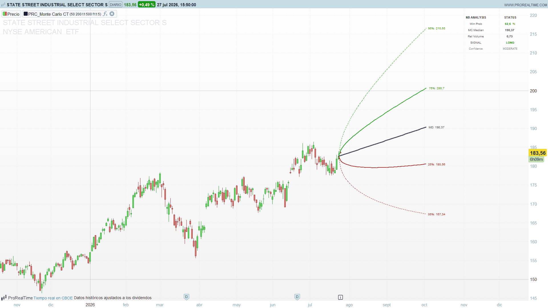
Most forecasting indicators draw a single line into the future and leave you to guess how much faith to put in it. This one draws five, and the distance between them is the message: a fan of price percentiles projected forward from the last closed bar, showing where price would end up in the 5%, 25%, 50%, 75% and 95% of scenarios under a model calibrated on the recent past.

Alongside it, a small panel runs a Gaussian Naive Bayes classifier on two features – relative volume and 10-bar momentum – and reports how the current bar looks against everything it has seen in its training window.

It is a price overlay and it works on any instrument and timeframe with enough history loaded.

2. The Model Behind the Fan

The fan assumes price follows a geometric Brownian motion: log returns are independent draws from a normal distribution whose mean and standard deviation are measured over the last lookBack bars.

Under that assumption the maths is closed. After t bars the log return is the sum of t independent normals, which is itself normal – with mean t * mu and variance t * sigma^2. So the percentile p of price at horizon t is simply:

price(t, p) = close * exp( t * mu + z(p) * sigma * sqrt(t) )

where z(p) is the standard normal quantile: 1.644854 for the 95th percentile, 0.674490 for the 75th, zero for the median, and the negatives of those for the 25th and 5th.

This is worth stating plainly, because it explains the shape you see on screen: the centre line drifts linearly with the horizon while the bands widen with its square root. Doubling the horizon doubles the drift but only widens the fan by a factor of 1.41. That square root is the single most useful thing the indicator tells you, and it is why the fan flares out instead of forming a cone with straight edges.

Evaluating the formula directly – rather than simulating thousands of random paths and taking sample percentiles of them – has two practical benefits. The bands come out perfectly smooth instead of wobbling with sampling noise, and the whole projection costs one pass of forecastLen iterations on the last bar, so you can push the horizon to several hundred bars without the chart slowing down.

3. The Naive Bayes Panel

The classifier is independent of the fan. It splits the last nbTrain bars into two classes – bars that closed up and bars that did not – and for each class it measures the mean and variance of two features:

• Relative volume: the bar’s volume divided by its 50-period average.
• Momentum: the 10-bar rate of change, in percent.

Each feature is then modelled as a Gaussian within each class, and the two likelihoods are combined with the class prior to produce a posterior probability for the current bar. The panel shows that probability, the median of the fan at the far end of the horizon, the current relative volume, the resulting LONG or SHORT reading, and a confidence tag that turns to HIGH once the probability leaves the 30-70% band.

Two implementation details are worth mentioning because they matter for robustness. The class statistics are accumulated with the native summation function over a per-class contribution series – each bar feeds its features into its own class and contributes zero to the other – so the whole sliding window costs no loops, no arrays and no recursion. And the posterior is evaluated in log space and closed with a sigmoid, which keeps it stable when both likelihoods become vanishingly small instead of collapsing to a meaningless zero.

4. Anchoring to the Last Closed Candle

Everything the indicator computes is anchored to the last closed candle, not to the bar currently forming. That is deliberate, and it matters as soon as the market is open.

A live bar has a provisional close that changes on every tick, so a fan anchored to it slides around continuously instead of standing still. Worse, the live bar also has a half-filled volume: a candle five minutes into a fifteen-minute period has accumulated roughly a third of the volume it will finish with, so its relative volume reads around 0.3x for purely mechanical reasons. Feed that into the classifier and the Win Prob drifts upward as the candle fills, which looks like information and is not.

Anchoring to the closed candle removes both problems at once – the projection is stable between ticks, and the classifier reads a feature that actually means something. The cost is that when the market is closed the fan starts one candle back instead of at the very last one, which is visually irrelevant. Set useClosedBar = 0 if you prefer the live-bar behaviour.

5. Parameters

• forecastLen (50) – how many bars the fan is projected forward. The chart needs enough right margin to show it.
• lookBack (200) – the window used to estimate drift and volatility.
• useDrift (1) – set to 0 to force the drift to zero. The fan then centres on the current price and shows volatility only. See the next section for why you may want this.
• useClosedBar (1) – anchor everything to the last closed candle. See section 4.
• nbTrain (500) – the classifier’s training window.
• lagFeatures (0) – set to 1 to train on the previous bar’s features against the current bar’s direction. See section 6.
• showPanel (1) – show or hide the statistics panel.
• showLabels (1) – show or hide the price label at the end of each band.

The indicator needs at least nbTrain + 62 bars of history before the panel appears, and lookBack + 1 before the fan is drawn.

Colours are set for the default light chart background. On a dark theme, swap the coloured(60, 60, 60) entries for coloured(255, 255, 255).

6. How to Read It Honestly

A projection this confident-looking deserves a warning label, so here are two, both of them measurable.

The drift is the noisiest part of the picture. The mean return mu is estimated from lookBack observations, so its standard error is sigma / sqrt(lookBack). In the projection that error gets multiplied by the horizon t, while the band half-width only grows with sqrt(t). Take the ratio and everything cancels except the two window lengths:

uncertainty in the drift        sqrt(t / lookBack)

————————  =  ———————-

   95% band half-width               1.645

With the defaults – a 50-bar horizon on a 200-bar lookback – the drift’s own error bar is already 30% of the band half-width. Push the horizon to 420 bars on the same lookback and it reaches 88%: at that point you are less sure about where the fan sits than about how wide it is. The tipping point is t / lookBack = 2.7; beyond it, the tilt of the median line carries essentially no information. This is what useDrift = 0 is for. Turning the drift off does not make the indicator less accurate – it makes it stop pretending to know something it does not.

The classifier describes the current bar rather than predicting the next one. By default, the class being learned is “this bar closed up” and both features are measured on that same bar – and one of them, 10-bar momentum, shares its closing price with the class label. The probability in the panel is therefore a statement about the bar you are already looking at, not a forecast. Set lagFeatures = 1 and the model trains on the previous bar’s features against the current bar’s direction, then evaluates today’s features to say something about tomorrow. That is a genuine one-bar-ahead prediction, and – as you would expect – a far less flattering number.

Used properly, the fan is a risk-sizing tool, not a direction tool: the 5% and 95% bands are a reasonable answer to “how far can this thing plausibly travel in the next N bars”, which is exactly what you need for stop placement and target setting. The direction reading belongs to the panel, and the panel is only as good as the caveat above allows.

7. Code

//-----------------------------------------------------------//
//PRC_Monte Carlo CT (by Steversteves)
//version = 1
//24.07.26
//Ivan Gonzalez @ www.prorealcode.com
//Sharing ProRealTime knowledge
//-----------------------------------------------------------//
// Projects a fan of price percentiles (5/25/50/75/95) N bars
// ahead under a GBM calibrated on the last "lookBack" log
// returns, and classifies the bar with a Gaussian Naive Bayes
// (relative volume + momentum).
// Everything is anchored to the last CLOSED candle: while the
// market is open the live bar has a provisional close and a
// half-filled volume.
//-----------------------------------------------------------//
defparam drawonlastbaronly = true
//-----Inputs------------------------------------------------//
forecastLen = 50     //Projection horizon in bars (2..500)
lookBack = 200       //Bars used to estimate drift and volatility
useDrift = 1         //1 = with drift, 0 = volatility only
useClosedBar = 1     //1 = anchor to the last closed candle, 0 = to the live bar
nbTrain = 500        //Naive Bayes training window
lagFeatures = 0      //1 = lag the features (true one-bar-ahead prediction)
showPanel = 1        //1 = show the Naive Bayes panel
showLabels = 1       //1 = price label at the end of each band
xoffset = 5
//-----------------------------------------------------------//

//-----1. GBM calibration (drift and volatility)-------------//
logRet = 0
if barindex > 0 and close > 0 and close[1] > 0 then
   logRet = log(close / close[1])
endif

muRaw = 0
sdRaw = 0
if barindex > lookBack then
   muRaw = average[lookBack](logRet)
   sdRaw = std[lookBack](logRet)
endif

// Shift one bar when anchoring to the closed candle, so the
// estimate excludes the live bar's provisional return.
if useClosedBar = 1 then
   muRet = muRaw[1]
   sdRet = sdRaw[1]
else
   muRet = muRaw
   sdRet = sdRaw
endif
if useDrift = 0 then
   muRet = 0
endif

//-----2. Naive Bayes features-------------------------------//
avgVol = average[50](volume)
relVol = 1.0
if barindex >= 50 and avgVol > 0 then
   relVol = volume / avgVol
endif

momPct = 0
if barindex >= 10 and close[10] > 0 then
   momPct = (close - close[10]) / close[10] * 100
endif

tgtUp = 0
if close > close[1] then
   tgtUp = 1
endif

// EVALUATION point. With useClosedBar = 1 the whole indicator
// reads the closed candle: the live bar's volume is only partly
// filled and drags relVol down mechanically, not informatively.
if useClosedBar = 1 then
   evV = relVol[1]
   evM = momPct[1]
   evT = tgtUp[1]
else
   evV = relVol
   evM = momPct
   evT = tgtUp
endif

// Features used for TRAINING. With lagFeatures = 1 they are
// lagged one more bar, so today's direction is learned from
// yesterday's features and the model really predicts.
if lagFeatures = 1 then
   trV = evV[1]
   trM = evM[1]
else
   trV = evV
   trM = evM
endif

//-----3. Per-class sliding window (native SUMMATION)--------//
// Each bar feeds its features into its own class and zero into
// the other one. summation[nbTrain] does the sliding window:
// no loops, no arrays, no recursive accumulators.
warmUp = 62
cvUp = 0
cqvUp = 0
cmUp = 0
cqmUp = 0
cvDn = 0
cqvDn = 0
cmDn = 0
cqmDn = 0
if evT = 1 then
   cvUp = trV
   cqvUp = trV * trV
   cmUp = trM
   cqmUp = trM * trM
else
   cvDn = trV
   cqvDn = trV * trV
   cmDn = trM
   cqmDn = trM * trM
endif

nUp = 0
nDn = 0
svUp = 0
qvUp = 0
smUp = 0
qmUp = 0
svDn = 0
qvDn = 0
smDn = 0
qmDn = 0
if barindex > warmUp + nbTrain then
   nUp = summation[nbTrain](evT)
   nDn = nbTrain - nUp
   svUp = summation[nbTrain](cvUp)
   qvUp = summation[nbTrain](cqvUp)
   smUp = summation[nbTrain](cmUp)
   qmUp = summation[nbTrain](cqmUp)
   svDn = summation[nbTrain](cvDn)
   qvDn = summation[nbTrain](cqvDn)
   smDn = summation[nbTrain](cmDn)
   qmDn = summation[nbTrain](cqmDn)
endif

//-----4. Gaussian posterior (in log space)------------------//
probUp = 0.5
nbReady = 0
if nUp >= 2 and nDn >= 2 then
   nbReady = 1
   mvUp = svUp / nUp
   vvUp = max(qvUp / nUp - mvUp * mvUp, 0.000001)
   mmUp = smUp / nUp
   vmUp = max(qmUp / nUp - mmUp * mmUp, 0.000001)
   mvDn = svDn / nDn
   vvDn = max(qvDn / nDn - mvDn * mvDn, 0.000001)
   mmDn = smDn / nDn
   vmDn = max(qmDn / nDn - mmDn * mmDn, 0.000001)
   
   piUp = nUp / (nUp + nDn)
   piUp = max(min(piUp, 0.999999), 0.000001)
   
   llUp = -0.5 * log(6.283185 * vvUp) - pow(evV - mvUp, 2) / (2 * vvUp)
   llUp = llUp - 0.5 * log(6.283185 * vmUp) - pow(evM - mmUp, 2) / (2 * vmUp)
   llUp = llUp + log(piUp)
   
   llDn = -0.5 * log(6.283185 * vvDn) - pow(evV - mvDn, 2) / (2 * vvDn)
   llDn = llDn - 0.5 * log(6.283185 * vmDn) - pow(evM - mmDn, 2) / (2 * vmDn)
   llDn = llDn + log(1 - piUp)
   
   dLL = llUp - llDn
   if dLL > 30 then
      probUp = 1
   elsif dLL < -30 then
      probUp = 0
   else
      probUp = 1 / (1 + exp(-dLL))
   endif
endif

//-----5. Percentile fan-------------------------------------//
// Normal quantiles: 95% = 1.644854, 75% = 0.674490
if islastbarupdate and sdRet > 0 and forecastLen >= 2 then
   // Anchor: price and index of the candle we project from
   if useClosedBar = 1 then
      p0 = close[1]
      xBase = barindex - 1
   else
      p0 = close
      xBase = barindex
   endif
   
   rndF = 100
   if p0 < 20 then
      rndF = 10000
   endif
   
   pv95 = p0
   pv75 = p0
   pv50 = p0
   pv25 = p0
   pv05 = p0
   
   for k = 1 to forecastLen - 1 do
      dK = muRet * k
      vK = sdRet * sqrt(k)
      n95 = p0 * exp(dK + 1.644854 * vK)
      n75 = p0 * exp(dK + 0.674490 * vK)
      n50 = p0 * exp(dK)
      n25 = p0 * exp(dK - 0.674490 * vK)
      n05 = p0 * exp(dK - 1.644854 * vK)
      xA = xBase + k - 1
      xB = xBase + k
      drawsegment(xA, pv95, xB, n95) coloured(0, 160, 0) style(dottedline, 1)
      drawsegment(xA, pv75, xB, n75) coloured(0, 160, 0) style(line, 2)
      drawsegment(xA, pv50, xB, n50) coloured(60, 60, 60) style(line, 3)
      drawsegment(xA, pv25, xB, n25) coloured(200, 0, 0) style(line, 2)
      drawsegment(xA, pv05, xB, n05) coloured(200, 0, 0) style(dottedline, 1)
      pv95 = n95
      pv75 = n75
      pv50 = n50
      pv25 = n25
      pv05 = n05
   next
   
   //-----6. Label at the end of each band-------------------//
   if showLabels = 1 then
      t95 = round(pv95 * rndF) / rndF
      t75 = round(pv75 * rndF) / rndF
      t50 = round(pv50 * rndF) / rndF
      t25 = round(pv25 * rndF) / rndF
      t05 = round(pv05 * rndF) / rndF
      xT = xBase + forecastLen
      drawtext("95%: #t95#", xT+xoffset, pv95, sansserif, standard, 10) anchor(topleft, index, value) coloured(0, 160, 0)
      drawtext("75%: #t75#", xT+xoffset, pv75, sansserif, standard, 10) anchor(topleft, index, value) coloured(0, 160, 0)
      drawtext("MD: #t50#", xT+xoffset, pv50, sansserif, standard, 10) anchor(topleft, index, value) coloured(60, 60, 60)
      drawtext("25%: #t25#", xT+xoffset, pv25, sansserif, standard, 10) anchor(topleft, index, value) coloured(200, 0, 0)
      drawtext("05%: #t05#", xT+xoffset, pv05, sansserif, standard, 10) anchor(topleft, index, value) coloured(200, 0, 0)
   endif
   
   //-----7. Naive Bayes panel-------------------------------//
   // pX is the distance in PIXELS to the window's right edge,
   // which includes the price scale - hence the wide margin.
   if showPanel = 1 and nbReady = 1 then
      pctUp = round(probUp * 1000) / 10
      medTg = round(p0 * exp(muRet * (forecastLen - 1)) * rndF) / rndF
      rvShow = round(evV * 100) / 100
      
      if probUp > 0.5 then
         pr = 0
         pg = 150
         pb = 0
      else
         pr = 200
         pg = 0
         pb = 0
      endif
      
      pX = -250
      pV = pX + 120
      pY = -30
      drawtext("NB ANALYSIS", pX, pY, sansserif, bold, 11) coloured(60, 60, 60) anchor(topright, xshift, yshift)
      drawtext("STATUS", pV, pY, sansserif, bold, 11) coloured(60, 60, 60) anchor(topright, xshift, yshift)
      
      drawtext("Win Prob", pX, pY - 22, sansserif, standard, 10) coloured(90, 90, 90) anchor(topright, xshift, yshift)
      drawtext("#pctUp# %", pV, pY - 22, sansserif, bold, 10) coloured(pr, pg, pb) anchor(topright, xshift, yshift)
      
      drawtext("MC Median", pX, pY - 44, sansserif, standard, 10) coloured(90, 90, 90) anchor(topright, xshift, yshift)
      drawtext("#medTg#", pV, pY - 44, sansserif, bold, 10) coloured(60, 60, 60) anchor(topright, xshift, yshift)
      
      drawtext("Rel Volume", pX, pY - 66, sansserif, standard, 10) coloured(90, 90, 90) anchor(topright, xshift, yshift)
      drawtext("#rvShow#", pV, pY - 66, sansserif, bold, 10) coloured(60, 60, 60) anchor(topright, xshift, yshift)
      
      drawtext("SIGNAL", pX, pY - 88, sansserif, standard, 10) coloured(90, 90, 90) anchor(topright, xshift, yshift)
      if probUp > 0.5 then
         drawtext("LONG", pV, pY - 88, sansserif, bold, 10) coloured(0, 150, 0) anchor(topright, xshift, yshift)
      else
         drawtext("SHORT", pV, pY - 88, sansserif, bold, 10) coloured(200, 0, 0) anchor(topright, xshift, yshift)
      endif
      
      drawtext("Confidence", pX, pY - 110, sansserif, standard, 9) coloured(130, 130, 130) anchor(topright, xshift, yshift)
      if probUp > 0.7 or probUp < 0.3 then
         drawtext("HIGH", pV, pY - 110, sansserif, standard, 9) coloured(130, 130, 130) anchor(topright, xshift, yshift)
      else
         drawtext("MODERATE", pV, pY - 110, sansserif, standard, 9) coloured(130, 130, 130) anchor(topright, xshift, yshift)
      endif
   endif
endif
//-----------------------------------------------------------//
//Drawing-only overlay: close with a bare RETURN
return