1. Introduction

Before taking a position it is worth asking a blunt question: if I buy here and hold for N bars, what is that trade worth on average? Not what the last signal did, not what the chart pattern suggests – the actual expected value, in currency, with the dispersion around it.

This indicator answers it twice, by two independent routes, and shows both answers side by side so you can see whether they agree.

The first route is empirical: it replays exactly that trade over and over through the recent history of the instrument and averages the results. The second is theoretical: it models price as a random walk calibrated on recent drift and volatility, and computes what such a walk implies for the same holding period.

It is a price overlay and works on any instrument and timeframe with enough history loaded.

2. The Empirical Estimate

The historical engine opens the same trade repeatedly. Starting histLookback bars back, it enters long, holds for tradeDuration bars, records the return, then steps forward and does it again. The step is one tenth of the holding period, so with the default settings you get 89 sampled trades over 2500 bars.

Optionally it applies a take profit and a stop loss. When useTPSL is set to 1 each trade is walked forward bar by bar and closed at whichever level is touched first, checking the stop before the target on each bar – the pessimistic convention, since a bar that spans both gives you no way to know which came first. Trades that reach neither level close at the end of the holding period.

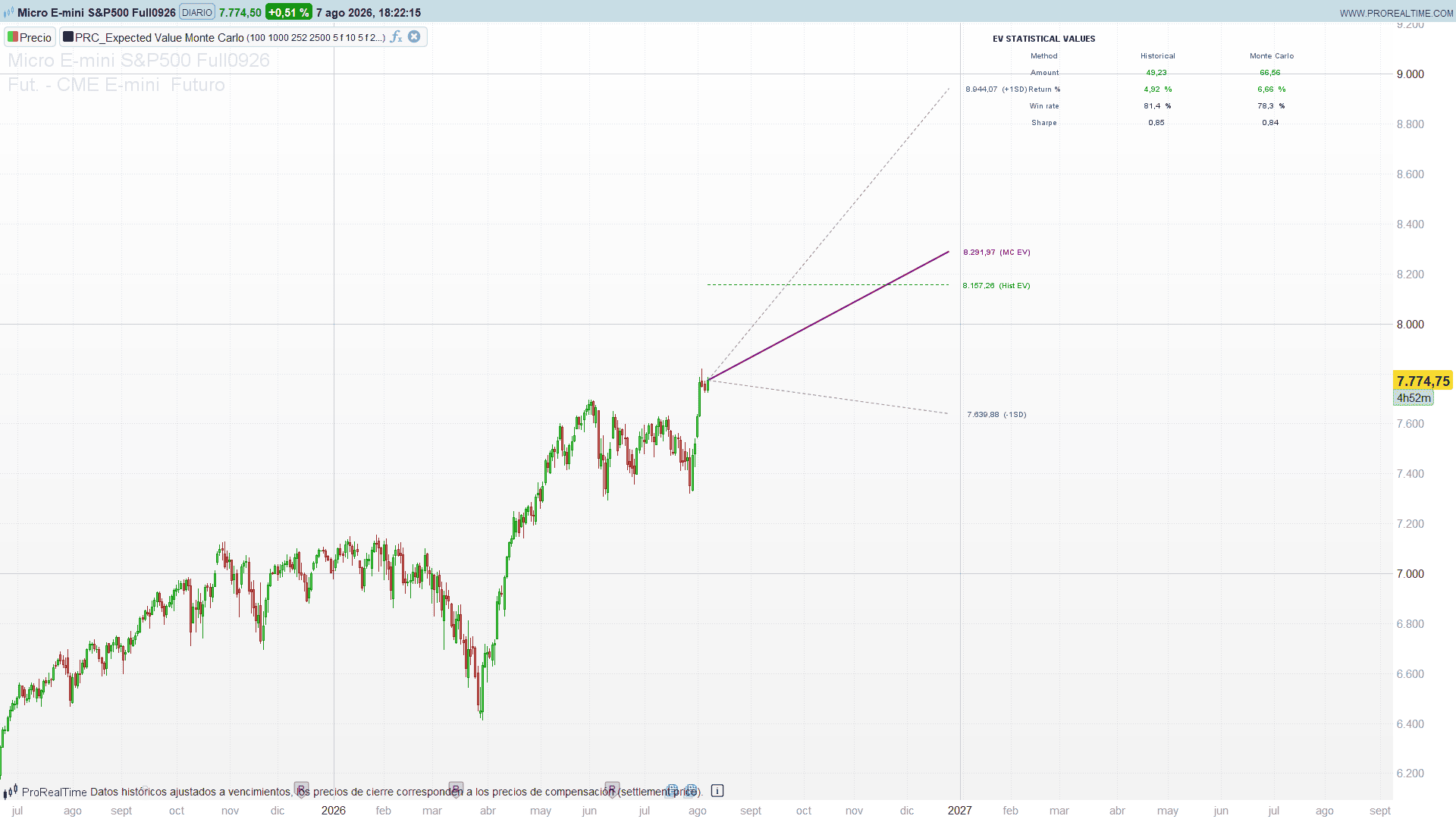
From the collection of returns it reports the mean (the expected value), the standard deviation, the proportion that finished positive, and an annualised Sharpe ratio.

3. The Theoretical Estimate

The second engine assumes log returns are independent draws from a normal distribution, with mean mu and standard deviation sigma measured over the last projLookback bars. That is the classic geometric Brownian motion.

Under that assumption, the total log return over N bars is the sum of N independent normals – which is itself normal, with mean mu*N and variance sigma^2 * N. The simple return of the trade is therefore:

R = exp(X) - 1        with X ~ Normal(m, s^2)
m = mu * N            s = sigma * sqrt(N)

R is a shifted lognormal, and everything the indicator needs from it has an exact formula:

expected value      E[R]  = exp(m + s^2/2) - 1
standard deviation  SD[R] = exp(m + s^2/2) * sqrt(exp(s^2) - 1)
probability of gain P(R>0) = Phi(m / s)

where Phi is the standard normal cumulative distribution, computed here with the Abramowitz and Stegun polynomial approximation – accurate to better than 1e-7, which is eight decimals more than a percentage needs.

This is worth dwelling on, because it is the whole reason the panel is stable. Simulating thousands of random paths and averaging them is an estimator of those three formulas. It converges to them, slowly, with an error that shrinks like one over the square root of the number of paths – and it lands on a slightly different number every time you run it. Evaluating the formulas directly gives you the value that the simulation is trying to approximate, exactly, at no computational cost. The figures in the panel move only when price or volatility move.

Note also what the s^2/2 term does. The expected simple return is not exp(m)-1; it sits above it, and the gap widens with volatility. That is the convexity of compounding, and it is why a volatile instrument can show a positive expected value on a flat drift.

4. When the Two Numbers Disagree

The two engines never talk to each other, and the interesting reading is in the gap between them.

The empirical figure carries everything the instrument actually did: trends, crashes, fat tails, the fact that big down days cluster together. The theoretical figure carries only two numbers, drift and volatility, and assumes every bar is an independent coin flip.

So when the historical expected value comes out far above the Monte Carlo one, the instrument trended more persistently than a random walk would – momentum that the model cannot see. When it comes out far below, the recent window has been kinder than the longer history, and the projection is extrapolating a good patch. When they roughly agree, a random walk is a fair description of what the instrument has been doing, and there is not much edge in the holding period itself.

The same logic applies to the win rates. The Monte Carlo win rate is a pure function of the ratio between drift and volatility. The historical one is a count. A large divergence between them tells you the return distribution is skewed – many small winners and a few large losers, or the reverse – which is precisely what a single expected value number hides.

5. Reading the Projection

To the right of the last price the indicator draws three lines out to tradeDuration bars:

• a solid purple line to the Monte Carlo expected value,
• two dotted grey lines to plus and minus one standard deviation of the simulated return.

That envelope is not a forecast of the path. It is the distribution of the endpoint: roughly two thirds of outcomes land between the dotted lines, and price is free to wander anywhere in between on the way there.

A dotted green horizontal line marks the historical expected value applied to the current price, which makes the gap discussed above visible at a glance rather than as two numbers in a panel.

6. Annualisation and the Sharpe Ratio

The Sharpe ratio needs an annual figure, so the indicator has to know how many bars make a year. That depends on the instrument and cannot be read from the chart directly, so it is set explicitly:

• assetType picks the calendar: 0 for stocks, forex and futures (252 trading days), 1 for crypto (365).
• sessionHours gives the length of the trading day, used only on intraday charts. Leave it at 24 for crypto and for any 24-hour market; set it to 6.5 for US equities, or whatever your session actually lasts.

Getting this wrong does not corrupt the whole panel – the expected values, the standard deviations and the win rates are all independent of it. It affects only the two Sharpe ratios. But it affects them substantially: assuming a 24-hour session on a 6.5-hour equity market overstates the annualised trend by a factor of 3.7 and the annualised volatility by 1.9, which roughly doubles the Sharpe ratio.

On daily charts and above the setting is ignored and the mapping is automatic: 252 or 365 bars a year for daily, 52 for weekly, 12 for monthly.

7. A Caveat Worth Knowing

The 89 sampled trades are not 89 independent observations. Consecutive samples overlap by 90% of their holding period, so they share most of their price history. Measured on daily US equity data, the correlation between one sampled trade and the next is around 0.75.

The number of genuinely independent trades is closer to histLookback / tradeDuration – about 10 with the default settings, not 89. That matters for how much weight to put on the historical column: a win rate of 87% measured on 10 independent trades carries an uncertainty of roughly plus or minus 10 percentage points, not the 3.5 that 89 samples would suggest.

This is not a defect to be fixed, it is the nature of overlapping-window sampling, and the alternative – stepping by the full holding period – would leave you with ten trades and an even noisier average. But it is the reason the historical Sharpe ratio should be read as an order of magnitude rather than a measurement, and why the divergence between the two engines is more informative than either number on its own.

8. Settings

• tradeDuration – holding period in bars, and the length of the projection.
• positionSize – position size in account currency; scales the amount and sigma figures.
• projLookback – bars used to calibrate drift and volatility. Shorter makes the projection more responsive to recent conditions and more prone to extrapolating them.
• histLookback – bars of history for the empirical engine. Must be at least tradeDuration + 50 or the historical column reports Raise lookback.
• riskFree – annual risk-free rate in percent, used only by the Sharpe ratios.
• useTPSL, tpPct, slPct – apply a take profit and stop loss to the historical trades.
• assetType, sessionHours – annualisation, see section 6.
• showProj, showLabels, showPanel – visibility toggles.
• panelX, panelY, panelCol – panel position and column spacing, in pixels from the top right corner of the window. Move the panel left by making panelX more negative if the price scale clips it on your screen.

Two practical notes. The projection extends tradeDuration bars to the right of the last price, which is 252 bars by default – you need that much free margin on the chart or you will not see it. And with useTPSL set to 1 the historical engine walks roughly 22,000 bars on every tick of the live candle, which can be noticeable on fast timeframes; leave it at 0 unless you need it.

9. The Code

//-----------------------------------------------------------//
//PRC_Expected Value Monte Carlo (by Henrique Centieiro)
//version = 1
//07.08.26
//Ivan Gonzalez @ www.prorealcode.com
//Sharing ProRealTime knowledge
//-----------------------------------------------------------//
// Two expected-value estimates for a long "buy and hold for N
// bars" trade, side by side:
//   1. HISTORICAL: replays the trade every "step" bars over the
//      last "histLookback" candles, optionally with TP/SL, and
//      averages the results.
//   2. MONTE CARLO: the same trade under a geometric brownian
//      motion calibrated on the last "projLookback" log returns.
//      Solved in CLOSED FORM (lognormal moments), so no random
//      number generator is needed and the figures never wobble.
// The projection is drawn to the right of the last price: mean
// path plus the one-standard-deviation cone.
//-----------------------------------------------------------//
defparam drawonlastbaronly = true
//-----Inputs (user settings)--------------------------------//
tradeDuration = 252   //Max trade duration in bars (1..)
positionSize = 1000   //Position size in account currency
projLookback = 252    //Bars used to calibrate drift and volatility (10..)
histLookback = 2500   //Bars of history for the backtest (1..5000)
riskFree = 5.0        //Annual risk-free rate (%), for the Sharpe ratio
useTPSL = 0           //1 = apply TP/SL to the historical trades
tpPct = 10.0          //Take profit (%)
slPct = 5.0           //Stop loss (%) 0.1..99.9
assetType = 0         //0 = stocks, forex, futures (252 days) / 1 = crypto (365 days)
sessionHours = 24     //Trading hours per day, intraday charts only. 24 = round-the-clock
showProj = 1          //1 = draw the projection to the right
showLabels = 1        //1 = price tags at the end of each line
showPanel = 1         //1 = statistics panel, top right
panelX = -540         //Panel offset in PIXELS from the right window edge
panelY = -20          //Panel offset in PIXELS from the top window edge
panelCol = 150        //Pixel gap between panel columns
//-----------------------------------------------------------//

//-----1. Bars per year (annualisation)-----------------------//
// The trading calendar cannot be read from the chart, so it is
// an input. On intraday charts a round-the-clock assumption
// overstates the bar count by 3.7x on a 6.5h equity session:
// sessionHours sets the real length of the session.
daysPerYear = 252
if assetType = 1 then
   daysPerYear = 365
endif

tfSec = gettimeframe
if tfSec < 86400 then
   barsPerYear = daysPerYear * sessionHours * 3600 / tfSec
elsif tfSec = 86400 then
   barsPerYear = daysPerYear
elsif tfSec = 604800 then
   barsPerYear = 52
else
   barsPerYear = 12
endif

//-----2. Drift and volatility of the log returns-------------//
logRet = 0
if barindex > 0 and close > 0 and close[1] > 0 then
   logRet = log(close / close[1])
endif

perBarDrift = 0
perBarVol = 0
if barindex > projLookback then
   perBarDrift = average[projLookback](logRet)
   perBarVol = std[projLookback](logRet)
endif

annTrend = perBarDrift * barsPerYear * 100
annVolPct = perBarVol * sqrt(barsPerYear) * 100

//-----3. Monte Carlo in closed form--------------------------//
// Every simulated path ends at R = exp(X) - 1 with
// X ~ Normal(drift * N, vol^2 * N). R is therefore LOGNORMAL and
// its mean, standard deviation and probability of being positive
// are exact formulas. Simulating only adds sampling noise.
mcReady = 0
mcEV = 0
mcEVpct = 0
mcSigma = 0
mcWin = 0
mcSharpe = 0
if perBarVol > 0 and tradeDuration >= 1 then
   mcReady = 1
   mDrift = perBarDrift * tradeDuration
   sVol = perBarVol * sqrt(tradeDuration)
   vTerm = sVol * sVol
   meanFactor = exp(mDrift + vTerm / 2)
   mcRet = meanFactor - 1
   mcSD = meanFactor * sqrt(exp(vTerm) - 1)
   
   // Win rate = P(X > 0) = Phi(mDrift / sVol).
   // Normal CDF via Abramowitz and Stegun 26.2.17, max error 7.5e-8.
   zArg = mDrift / sVol
   zAbs = abs(zArg)
   tCdf = 1 / (1 + 0.2316419 * zAbs)
   dCdf = 0.3989422804 * exp(-zAbs * zAbs / 2)
   pCdf = tCdf * (0.319381530 + tCdf * (-0.356563782 + tCdf * (1.781477937 + tCdf * (-1.821255978 + tCdf * 1.330274429))))
   upTail = 1 - dCdf * pCdf
   if zArg >= 0 then
      mcWin = upTail * 100
   else
      mcWin = (1 - upTail) * 100
   endif
   
   mcEV = mcRet * positionSize
   mcEVpct = mcRet * 100
   mcSigma = mcSD * positionSize
   if annVolPct > 0 then
      mcSharpe = (annTrend - riskFree) / annVolPct
   endif
endif

//-----4. Historical backtest---------------------------------//
// Re-enters the same trade every "stepSize" bars and averages the
// outcomes. Mean and variance come from one single pass using
// E[x^2] - E[x]^2, so the TP/SL scan is not walked twice.
histReady = 0
lowLookback = 0
histEV = 0
histEVpct = 0
histSigma = 0
histWin = 0
histSharpe = 0
if islastbarupdate then
   if histLookback < tradeDuration + 50 then
      lowLookback = 1
   else
      stepSize = max(3, floor(tradeDuration / 10))
      nSteps = floor((histLookback - tradeDuration - stepSize) / stepSize)
      cnt = 0
      sumRet = 0
      sumSq = 0
      winCnt = 0
      if nSteps >= 0 then
         for j = 0 to nSteps do
            entryAgo = tradeDuration + stepSize + j * stepSize
            if barindex > entryAgo then
               entryP = close[entryAgo]
               tradeRet = 0
               if useTPSL = 0 then
                  exitP = close[entryAgo - tradeDuration]
                  tradeRet = (exitP - entryP) / entryP
               else
                  tpLevel = entryP * (1 + tpPct / 100)
                  slLevel = entryP * (1 - slPct / 100)
                  exitFound = 0
                  exitP = 0
                  for i = 1 to tradeDuration do
                     barOff = entryAgo - i
                     if low[barOff] <= slLevel then
                        exitP = slLevel
                        exitFound = 1
                        break
                     endif
                     if high[barOff] >= tpLevel then
                        exitP = tpLevel
                        exitFound = 1
                        break
                     endif
                  next
                  if exitFound = 0 then
                     exitP = close[entryAgo - tradeDuration]
                  endif
                  tradeRet = (exitP - entryP) / entryP
               endif
               cnt = cnt + 1
               sumRet = sumRet + tradeRet
               sumSq = sumSq + tradeRet * tradeRet
               if tradeRet > 0 then
                  winCnt = winCnt + 1
               endif
            endif
         next
      endif
      
      if cnt > 0 then
         histReady = 1
         avgRet = sumRet / cnt
         vRet = max(sumSq / cnt - avgRet * avgRet, 0)
         periodVol = sqrt(vRet)
         histEV = avgRet * positionSize
         histEVpct = avgRet * 100
         histSigma = periodVol * positionSize
         histWin = winCnt / cnt * 100
         annVolH = periodVol * sqrt(barsPerYear / tradeDuration) * 100
         if 1 + avgRet > 0 and annVolH > 0 then
            annRetH = (pow(1 + avgRet, barsPerYear / tradeDuration) - 1) * 100
            histSharpe = (annRetH - riskFree) / annVolH
         endif
      endif
   endif
endif

//-----5. Drawing---------------------------------------------//
if islastbarupdate then
   entryPrice = close
   xEnd = barindex + tradeDuration
   rndF = 100
   if entryPrice < 20 then
      rndF = 10000
   endif
   
   //-----5a. Monte Carlo cone--------------------------------//
   if showProj = 1 and mcReady = 1 then
      sdPct = mcSigma / positionSize * 100
      evPrice = entryPrice * (1 + mcEVpct / 100)
      upPrice = entryPrice * (1 + (mcEVpct + sdPct) / 100)
      dnPrice = entryPrice * (1 + (mcEVpct - sdPct) / 100)
      drawsegment(barindex, entryPrice, xEnd, evPrice) coloured(128, 0, 128) style(line, 2)
      drawsegment(barindex, entryPrice, xEnd, upPrice) coloured(130, 130, 130) style(dottedline, 1)
      drawsegment(barindex, entryPrice, xEnd, dnPrice) coloured(130, 130, 130) style(dottedline, 1)
      if showLabels = 1 then
         tUp = round(upPrice * rndF) / rndF
         tEv = round(evPrice * rndF) / rndF
         tDn = round(dnPrice * rndF) / rndF
         drawtext("#tUp# (+1SD)", xEnd+20, upPrice, sansserif, standard, 10) anchor(topleft, index, value) coloured(90, 90, 90)
         drawtext("#tEv# (MC EV)", xEnd+20, evPrice, sansserif, bold, 10) anchor(topleft, index, value) coloured(128, 0, 128)
         drawtext("#tDn# (-1SD)", xEnd+20, dnPrice, sansserif, standard, 10) anchor(topleft, index, value) coloured(90, 90, 90)
      endif
   endif
   
   //-----5b. Historical EV level-----------------------------//
   if showProj = 1 and histReady = 1 then
      histPrice = entryPrice * (1 + histEVpct / 100)
      drawsegment(barindex, histPrice, xEnd, histPrice) coloured(0, 150, 0) style(dottedline, 1)
      if showLabels = 1 then
         tHist = round(histPrice * rndF) / rndF
         drawtext("#tHist# (Hist EV)", xEnd+20, histPrice, sansserif, standard, 10) anchor(topleft, index, value) coloured(0, 150, 0)
      endif
   endif
   
   //-----5c. Statistics panel--------------------------------//
   // The panel is built with DRAWTEXT anchored in PIXELS from the
   // top right corner of the WINDOW, which includes the price
   // scale: hence the wide margins.
   if showPanel = 1 then
      hx = panelX + panelCol
      mx = panelX + panelCol * 2
      
      if useTPSL = 1 then
         drawtext("EV STATISTICAL VALUES (TP/SL)", panelX, panelY, sansserif, bold, 11) coloured(60, 60, 60) anchor(topright, xshift, yshift)
      else
         drawtext("EV STATISTICAL VALUES", panelX, panelY, sansserif, bold, 11) coloured(60, 60, 60) anchor(topright, xshift, yshift)
      endif
      drawtext("Method", panelX, panelY - 22, sansserif, bold, 10) coloured(90, 90, 90) anchor(topright, xshift, yshift)
      drawtext("Historical", hx, panelY - 22, sansserif, bold, 10) coloured(90, 90, 90) anchor(topright, xshift, yshift)
      drawtext("Monte Carlo", mx, panelY - 22, sansserif, bold, 10) coloured(90, 90, 90) anchor(topright, xshift, yshift)
      
      drawtext("Amount", panelX, panelY - 44, sansserif, standard, 10) coloured(90, 90, 90) anchor(topright, xshift, yshift)
      drawtext("Return %", panelX, panelY - 66, sansserif, standard, 10) coloured(90, 90, 90) anchor(topright, xshift, yshift)
      drawtext("Win rate", panelX, panelY - 88, sansserif, standard, 10) coloured(90, 90, 90) anchor(topright, xshift, yshift)
      drawtext("Sharpe", panelX, panelY - 110, sansserif, standard, 10) coloured(90, 90, 90) anchor(topright, xshift, yshift)
      
      // Historical column
      if lowLookback = 1 then
         drawtext("Raise lookback", hx, panelY - 44, sansserif, standard, 10) coloured(220, 130, 0) anchor(topright, xshift, yshift)
      elsif histReady = 0 then
         drawtext("No data", hx, panelY - 44, sansserif, standard, 10) coloured(130, 130, 130) anchor(topright, xshift, yshift)
      else
         hr = 200
         hg = 0
         hb = 0
         if histEV >= 0 then
            hr = 0
            hg = 150
            hb = 0
         endif
         vhAmt = round(histEV * 100) / 100
         vhRet = round(histEVpct * 100) / 100
         vhWin = round(histWin * 10) / 10
         vhShp = round(histSharpe * 100) / 100
         drawtext("#vhAmt#", hx, panelY - 44, sansserif, bold, 10) coloured(hr, hg, hb) anchor(topright, xshift, yshift)
         drawtext("#vhRet# %", hx, panelY - 66, sansserif, bold, 10) coloured(hr, hg, hb) anchor(topright, xshift, yshift)
         drawtext("#vhWin# %", hx, panelY - 88, sansserif, standard, 10) coloured(60, 60, 60) anchor(topright, xshift, yshift)
         drawtext("#vhShp#", hx, panelY - 110, sansserif, standard, 10) coloured(60, 60, 60) anchor(topright, xshift, yshift)
      endif
      
      // Monte Carlo column
      if mcReady = 0 then
         drawtext("No data", mx, panelY - 44, sansserif, standard, 10) coloured(130, 130, 130) anchor(topright, xshift, yshift)
      else
         mr = 200
         mg = 0
         mb = 0
         if mcEV >= 0 then
            mr = 0
            mg = 150
            mb = 0
         endif
         vmAmt = round(mcEV * 100) / 100
         vmRet = round(mcEVpct * 100) / 100
         vmWin = round(mcWin * 10) / 10
         vmShp = round(mcSharpe * 100) / 100
         drawtext("#vmAmt#", mx, panelY - 44, sansserif, bold, 10) coloured(mr, mg, mb) anchor(topright, xshift, yshift)
         drawtext("#vmRet# %", mx, panelY - 66, sansserif, bold, 10) coloured(mr, mg, mb) anchor(topright, xshift, yshift)
         drawtext("#vmWin# %", mx, panelY - 88, sansserif, standard, 10) coloured(60, 60, 60) anchor(topright, xshift, yshift)
         drawtext("#vmShp#", mx, panelY - 110, sansserif, standard, 10) coloured(60, 60, 60) anchor(topright, xshift, yshift)
      endif
   endif
endif
//-----------------------------------------------------------//
return