Hola Nicolas,

A ver si es tan amable de traducir el código a PRT.Creo que será útil y novedoso sobretodo para los amantes de las redes neuronales…

Un saludo

Notas del autor:

NOTA IMPORTANTE: Si se utiliza la función de activación tangente, los datos de entrada también deben tener valores tangentes (en comparación con los valores anteriores de 1 bar). Los insumos fueron preparados de acuerdo con este juicio.

1. La función tangente que es la función de activación está escrita correctamente. (La función tangente en el artículo: ActivationFunctionTanh (v) => (1 – exp (-2 * v)) / (1 + exp (-2 * v)))

2. Se agregaron partes de sesgo faltantes en las fórmulas.

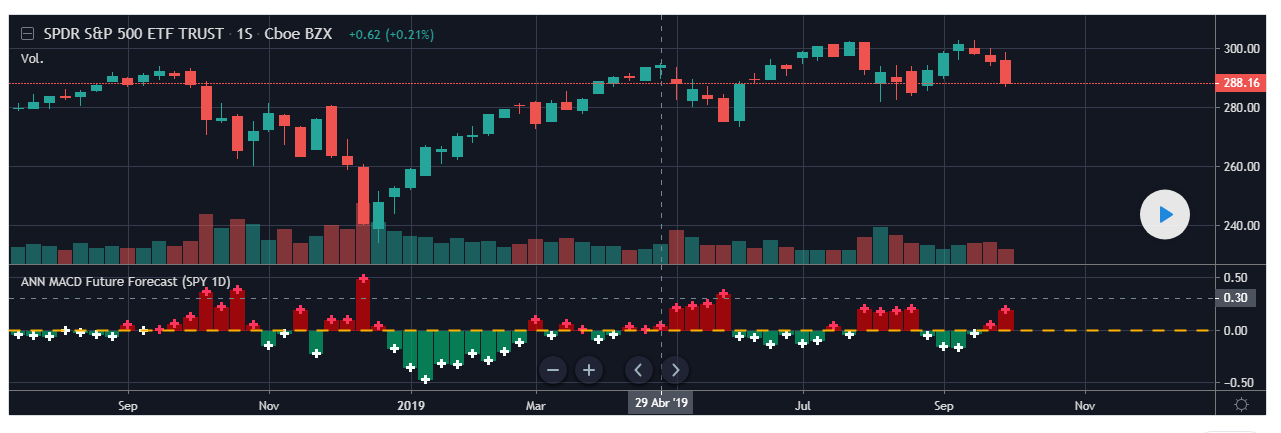
3. La función de salida se toma del día siguiente (histórico), de modo que se pueda predecir la siguiente barra, que es la verdad.

4. El valor de pronóstico de la siguiente barra se resta del cambio de barra actual y se determina la dirección del mercado.

5. Cuando el pronóstico futuro y el cierre actual se suman, los datos resultantes se denominan semilla. La semilla lleva datos tanto del presente como del ayer y del futuro.

6. Y esta semilla fue sometida al método MACD. Por lo tanto, debido a promedios exponenciales, se dará más importancia a los desarrollos recientes y Las situaciones de aceleración nos mostrarán la dirección. Sin embargo, se debe tomar una posición corta para el cruce y una posición larga para el cruce. Porque los valores pronosticados funcionan al revés. ¡Aunque usamos el mismo período (9,12,26) es mucho más rápido!

7. No existe un código futuro que pueda causar el repintado. Sin embargo, se debe verificar el color después del cierre. El sistema es completamente correcto. Sin embargo, se seleccionó una muestra muy estrecha.

//@version=4

//MIT License

//Copyright (c) 2019 user-Noldo

//Permission is hereby granted, free of charge, to any person obtaining a copy
//of this software and associated documentation files (the "Software"), to deal
//in the Software without restriction, including without limitation the rights
//to use, copy, modify, merge, publish, distribute, sublicense, and/or sell
//copies of the Software, and to permit persons to whom the Software is
//furnished to do so, subject to the following conditions:

//The above copyright notice and this permission notice shall be included in all
//copies or substantial portions of the Software.

//THE SOFTWARE IS PROVIDED "AS IS", WITHOUT WARRANTY OF ANY KIND, EXPRESS OR
//IMPLIED, INCLUDING BUT NOT LIMITED TO THE WARRANTIES OF MERCHANTABILITY,
//FITNESS FOR A PARTICULAR PURPOSE AND NONINFRINGEMENT. IN NO EVENT SHALL THE
//AUTHORS OR COPYRIGHT HOLDERS BE LIABLE FOR ANY CLAIM, DAMAGES OR OTHER
//LIABILITY, WHETHER IN AN ACTION OF CONTRACT, TORT OR OTHERWISE, ARISING FROM,
//OUT OF OR IN CONNECTION WITH THE SOFTWARE OR THE USE OR OTHER DEALINGS IN THE
//SOFTWARE.


study("ANN MACD Future Forecast (SPY 1D) ", max_bars_back=21)
src = close[0]

lights          = input(title="Barcolor I / 0 ? ", options=["ON", "OFF"], defval="OFF")


// Essential Functions

// Highest - Lowest Functions ( All efforts goes to RicardoSantos )

f_highest(_src, _length)=>
    _adjusted_length = _length < 1 ? 1 : _length
    _value = _src
    for _i = 0 to (_adjusted_length-1)
        _value := _src[_i] >= _value ? _src[_i] : _value
    _return = _value

f_lowest(_src, _length)=>
    _adjusted_length = _length < 1 ? 1 : _length
    _value = _src
    for _i = 0 to (_adjusted_length-1)
        _value := _src[_i] <= _value ? _src[_i] : _value
    _return = _value

// Function Sum  

f_sum(_src , _length) => 

    _output  = 0.00 
    
    _length_adjusted = _length < 1 ? 1 : _length
    
    for i = 0 to _length_adjusted-1
        _output := _output + _src[i]


// Unlocked Exponential Moving Average Function

f_ema(_src, _length)=>
    _length_adjusted = _length < 1 ? 1 : _length
    _multiplier = 2 / (_length_adjusted + 1)
    _return  = 0.00
    _return := na(_return[1]) ? _src : ((_src - _return[1]) * _multiplier) + _return[1]


// Unlocked Moving Average Function 

f_sma(_src, _length)=>
    
    _output = 0.00
    _length_adjusted = _length < 0 ? 0 : _length
    w = cum(_src)

    _output:= (w - w[_length_adjusted]) / _length_adjusted
   
    _output    


// Definition : Function Bollinger Bands

Multiplier = 2 
_length_bb = 20


e_r = f_sma(src,_length_bb)


// Function Standard Deviation : 

f_stdev(_src,_length) =>

    float _output = na 
    _length_adjusted = _length < 2 ? 2 : _length
    _avg  = f_ema(_src , _length_adjusted)
    evar  = (_src - _avg) * (_src - _avg)
    evar2 = ((f_sum(evar,_length_adjusted))/_length_adjusted)
    
    _output := sqrt(evar2)


std_r = f_stdev(src , _length_bb )


upband = e_r + (Multiplier * std_r)  // Upband
dnband = e_r - (Multiplier * std_r)  // Lowband
basis  = e_r                         // Midband

// Function : Squeeze Momentum Indicator (SQZMOM_LB) (LazyBear)

length = 20
mult = 2.0
lengthKC=20
multKC = 1.5

// Calculate BB

dev = multKC * f_stdev(src, length)
upperBB = e_r + dev
lowerBB = e_r - dev

// Calculate KC

ma = f_sma(src, lengthKC)
range = tr
rangema = f_sma(range, lengthKC)
upperKC = ma + rangema * multKC
lowerKC = ma - rangema * multKC

sqzOn  = (lowerBB > lowerKC) and (upperBB < upperKC)
sqzOff = (lowerBB < lowerKC) and (upperBB > upperKC)
noSqz  = (sqzOn == false) and (sqzOff == false)

val = linreg(src -  f_sma(f_sma(f_highest(f_highest(src,1), lengthKC), f_lowest(f_lowest(src,1), lengthKC)),f_sma(src,lengthKC)), lengthKC,0)


// Inputs on Tangent Function : 

tangentdiff(_src) => nz((_src - _src[1]) / _src[1] ) 


// Deep Learning Activation Function (Tanh) : 

ActivationFunctionTanh(v) => (1 - exp(-2 * v))/( 1 + exp(-2 * v))


// DEEP LEARNING 

// INPUTS : 

input_1 = tangentdiff(volume)
input_2 = tangentdiff(e_r)
input_3 = tangentdiff(upband)
input_4 = tangentdiff(dnband)
input_5 = tangentdiff(val)


// LAYERS : 

// Input Layers 

n_0 = ActivationFunctionTanh(input_1 + 0)   
n_1 = ActivationFunctionTanh(input_2 + 0) 
n_2 = ActivationFunctionTanh(input_3 + 0) 
n_3 = ActivationFunctionTanh(input_4 + 0) 
n_4 = ActivationFunctionTanh(input_5 + 0) 


// Hidden Layers 

n_5  = ActivationFunctionTanh( -35.733   * n_0 + -86.718  * n_1 + -16.948 * n_2 +  -12.384  * n_3 + -38.803  * n_4 +  43.379) 
n_6  = ActivationFunctionTanh(  -2.394   * n_0 + -85.060  * n_1 +  -6.174 * n_2 +  -45.667  * n_3 +  26.925  * n_4 +  16.028) 
n_7  = ActivationFunctionTanh( -63.221   * n_0 +  -7.447  * n_1 +  34.106 * n_2 +  -28.880  * n_3 + -23.098  * n_4 +   9.914) 
n_8  = ActivationFunctionTanh( -59.117   * n_0 +  41.706  * n_1 +  19.044 * n_2 +  -13.141  * n_3 +  40.028  * n_4 + -50.017) 
n_9  = ActivationFunctionTanh( -9.193    * n_0 +  -64.825 * n_1 +  12.735 * n_2 +  11.168   * n_3 +  13.162  * n_4 +  -6.669) 


// Output Layer 

_output  = ActivationFunctionTanh(4.118 * n_5 + 36.306 * n_6 + -22.908 * n_7 + 11.143 * n_8 + -32.203 * n_9  + -0.263)

_chg_src = tangentdiff(src) * 100

_seed = (_output - _chg_src)


// MACD : SEED 


fastLength   = 12
slowlength   = 26
signalLength = 9


macd   = f_ema(_seed, fastLength) - f_ema(_seed, slowlength)
signal = f_ema(macd, signalLength)
	   

hist = macd - signal

// Conditions : 

positive_condition = hist < 0 
negative_condition = hist > 0

col_hist() => positive_condition ? color.new(#F5FFFA,0) : negative_condition ? color.new(#FF355E,0) : color.new(color.yellow,0)
col_histo = col_hist()

//Plot data

hline(0, color=#FFB300, linewidth = 2)

plot(hist, color=(positive_condition ? #00A86B : #D40000), style=plot.style_columns,linewidth= 5 , title="Area", transp=30)
plot(hist, color=col_histo,style =plot.style_cross, title="Forecast", linewidth=3)



// Definition : Barcolor 

_lights = 0.00 


if (lights=="ON")

    _lights:= 1.00
    
if (lights=="OFF")

    _lights:= -1.00   


bcolor_on  = _lights ==  1.00
bcolor_off = _lights == -1.00


color_condition() => 

    (positive_condition and _lights == 1.00) ?  color.green  : (negative_condition and _lights == 1.00)  ?  color.red : na 
   
  
color barColor = na 
barColor := color_condition()

barcolor(color = barColor)

ANN-MACD.png