Introduction

Most composite oscillators blend a handful of indicators with fixed, hand-picked weights. Neural Weight Oscillator, by Zeiierman, replaces that guesswork with two ideas borrowed from operations research and machine learning. First, it decides how much each component matters with the Best-Worst Method (BWM) — a structured multi-criteria decision technique where you only declare which factor is most important, which is least, and how they compare. Second, it adds an online learning layer that nudges those weights bar by bar, using a small gradient-descent optimizer. The output is a single, bounded 0-100 oscillator that fuses trend, mean-reversion and momentum into one transparent line. This article explains exactly what each layer does — including an honest look at how much the “learning” layer really contributes — and gives you the full ProBuilder translation.

Theory Behind the Indicator

Three normalized components

The oscillator starts from three classic readings, each squeezed into a 0-100 range:

• Trend — the spread between a fast and a slow EMA plus the fast EMA’s slope, both divided by ATR so the reading is volatility-adjusted and comparable across instruments.
• Mean Reversion — the inverted RSI (100 − RSI) averaged with the inverted price z-score over its moving average. High when price is stretched below its mean, low when overextended above.
• Momentum — a blend of rate-of-change, RSI and the ATR-normalized EMA slope.

Each is then centered into a feature in [-1, +1] (0 at the neutral 50 level). These three features are the raw material everything else works on.

The Best-Worst Method

How do you weight trend versus mean-reversion versus momentum? The BWM (Rezaei, 2015) is a lightweight multi-criteria decision method that needs only two comparison vectors:

• Best-to-Others (BO): pick the single most important criterion (the Best), then rate how much more important it is than each of the others, on a 1-9 scale.
• Relative-to-Worst (OW): pick the least important criterion (the Worst), then rate how much more important each criterion is than that one.

From those two vectors the method derives a consistent set of weights. This implementation uses the closed-form estimate w_i = sqrt((a_BW / bo_i) · ow_i), normalized to sum to 1, where a_BW is the Best-to-Others score of the Worst criterion. With the defaults — Trend as Best, Momentum as Worst — the weights come out roughly Trend 0.64 / Mean-Reversion 0.26 / Momentum 0.11. The elegance is that you never assign raw weights by hand; you express preferences and the method turns them into numbers.

The online learning layer

On top of the fixed BWM weights sits an adaptive layer. Every bar it fits a tiny linear model — prediction = w_trend·trend + w_mean·mean + w_momentum·momentum + bias — whose four parameters are trained by the Adam optimizer (with a Huber loss) to predict the direction of price a few bars ahead. The learned weights are then used two ways: they amplify each component (a factor between roughly 0.7 and 1.3) and they shift the oscillator line slightly toward the model’s own prediction. Both effects are deliberately capped, so the learning layer modulates the oscillator rather than dominating it.

A word of realism, since the name invites big expectations: this is a single-layer linear model with no hidden layers and no non-linear activation — mathematically, an adaptively-weighted regression, not a neural network. Its target (the sign of a short-horizon return) is close to noise in most markets, and it learns online with no out-of-sample validation. In practice the deterministic BWM core drives well over 90% of the oscillator’s value; the adaptive layer is a light, self-adjusting overlay. It is a genuinely adaptive weighting scheme — just not the black-box brain the label might suggest.

Signal line, histogram and liquidity sweeps

The oscillator is finished with an EMA signal line, a momentum histogram plotted around the 50 midline, and crossover signals gated by a simple liquidity-sweep filter: a bullish signal requires the oscillator to cross up through its signal line while below 30, right after price swept a prior low and closed back above it (the bearish case mirrors this above 70).

How to Read the Indicator

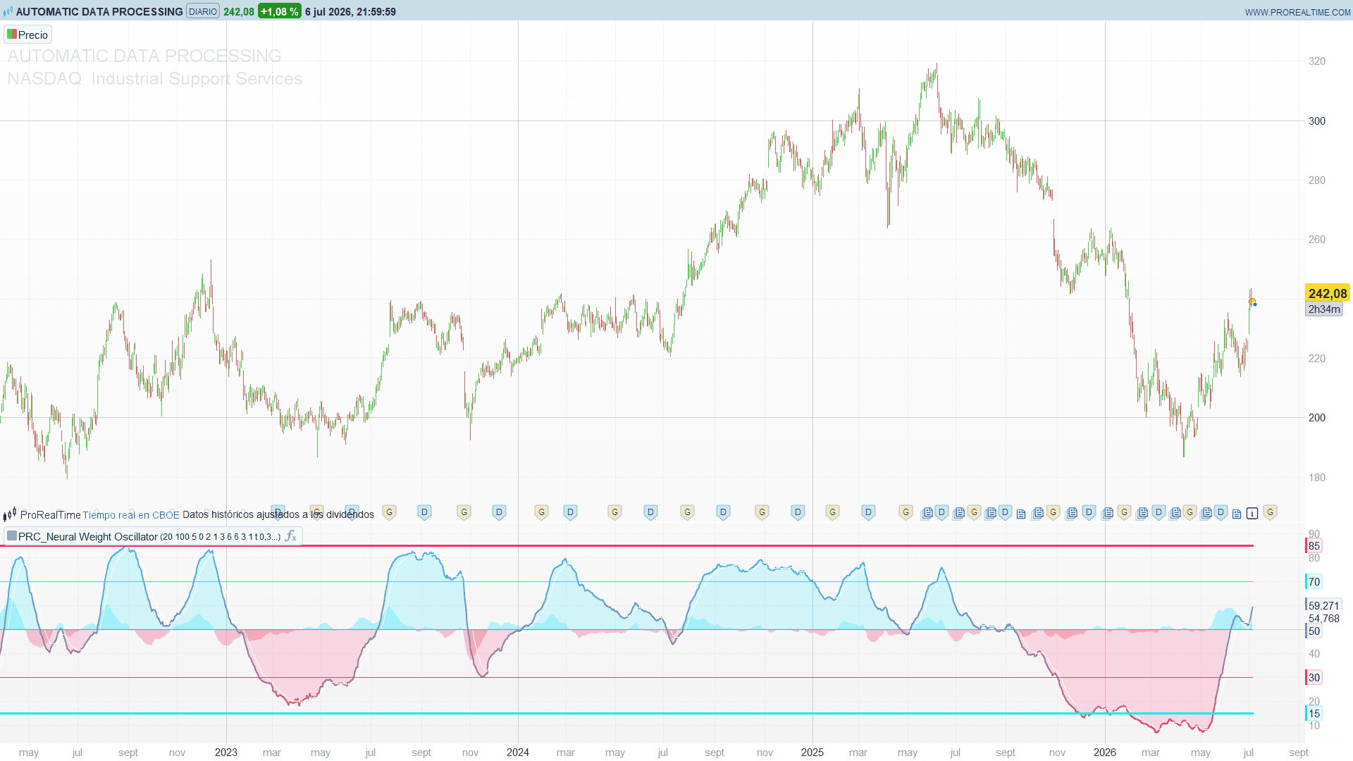
1. 50 is the pivot. Above 50 the weighted blend leans bullish, below 50 bearish. The line’s color runs on a gradient from bearish (below) to bullish (above).
2. Overbought / oversold zones. 70 and 30 are the primary bands (80/20 as extremes). Readings inside the outer zones flag stretched conditions.
3. Signal-line crossovers are the momentum trigger; the histogram around 50 shows the oscillator pulling away from or converging on its signal line.
4. Marked signals (the plotted points near the top and bottom) are the highest-conviction events: an oscillator crossover in an extreme zone confirmed by a recent liquidity sweep.
5. Toggle the learning layer. Set useTraining to 0 to see the pure BWM oscillator, and to 1 to add the adaptive modulation — a useful A/B test to judge for yourself how much the learning layer changes on your instrument.

Practical Applications

1. Transparent component blending. Use the BWM inputs to encode your market view — if you trade a trending instrument, keep Trend as Best; for a range, promote Mean Reversion — and let the method produce consistent weights instead of hand-tuned ones.
2. Confluence filter. Because the oscillator already fuses trend, mean-reversion and momentum, a single reading above/below 50 is a compact regime filter for entries taken from another system.
3. Extreme-zone reversals. The sweep-confirmed marked signals in the 30/70 zones are candidate mean-reversion entries; treat them as alerts, not standalone triggers.
4. Adaptive-vs-fixed study. The useTraining switch makes this a clean teaching tool for what an online learning layer actually adds to a rule-based indicator.

Indicator Configuration

• lenFast / lenSlow (20 / 100): fast and slow EMAs feeding the trend and momentum components.
• smoothLen (5): final smoothing of the oscillator line.
• bestCrit / worstCrit (0 / 2): the Best and Worst criteria (0 = Trend, 1 = Mean Reversion, 2 = Momentum).
• boTrend / boMean / boMomentum (1 / 3 / 6): the Best-to-Others comparison vector (the Best criterion’s own entry should be 1).
• owTrend / owMean / owMomentum (6 / 3 / 1): the Relative-to-Worst comparison vector (the Worst criterion’s own entry should be 1).
• useTraining (1): enable the adaptive Adam layer; 0 leaves the pure BWM oscillator.
• learnInfluence (0.30): how strongly the learned weights amplify each component.
• lineInfluence (0.25): how strongly the learned model shifts the oscillator line.
• signalLen (9): length of the signal-line EMA.
• showGradient / showHistogram / showSignals (1): visual toggles.

Code

//----------------------------------------------
//PRC_Neural Weight Oscillator
//version = 0
//07.07.2026
//Iván González @ www.prorealcode.com
//Translated from "Neural Weight Oscillator (Zeiierman)" (PineScript v6)
//Original author: Zeiierman
//Sharing ProRealTime knowledge
//----------------------------------------------
// === Inputs ===
//----------------------------------------------
lenFast = 20         // EMA rapida (trend + momentum)
lenSlow = 100        // EMA lenta (baseline de tendencia)
smoothLen = 5        // suavizado final del oscilador
bestCrit = 0         // criterio Best  : 0=Trend 1=MeanRev 2=Momentum
worstCrit = 2        // criterio Worst : 0=Trend 1=MeanRev 2=Momentum
boTrend = 1          // Best-to-Others: Trend
boMean = 3           // Best-to-Others: Mean Reversion
boMomentum = 6       // Best-to-Others: Momentum
owTrend = 6          // Relative-to-Worst: Trend
owMean = 3           // Relative-to-Worst: Mean Reversion
owMomentum = 1       // Relative-to-Worst: Momentum
useTraining = 1      // 1 = activar capa adaptativa Adam, 0 = solo BWM
learnInfluence = 0.30 // cuanto amplifica el modelo aprendido a los features
lineInfluence = 0.25  // cuanto desplaza el modelo aprendido a la linea
signalLen = 9        // longitud de la linea de senal
showGradient = 1     // 1 = relleno tendencial alrededor del oscilador
showHistogram = 1    // 1 = histograma de momentum alrededor de 50
showSignals = 1      // 1 = marcas de cruce oscilador/senal
//----------------------------------------------
// === Constantes internas ===
lenRSI = 14
lenATR = 14
lenMomentum = 20
warmupBars = 100
targetLen = 3
lrate = 0.01
huberD = 0.01
beta1 = 0.9
beta2 = 0.999
epsv = 0.00000001
aiCenterLen = 100
histSmooth = 3
//----------------------------------------------
// === BWM (Best-Worst Method) - pesos de los 3 criterios ===
$bo[0] = boTrend
$bo[1] = boMean
$bo[2] = boMomentum
$ow[0] = owTrend
$ow[1] = owMean
$ow[2] = owMomentum
$bo[bestCrit] = 1.0
$ow[worstCrit] = 1.0
aBW = $bo[worstCrit]
totalW = 0
for i = 0 to 2 do
   $wt[i] = sqrt((aBW / $bo[i]) * $ow[i])
   totalW = totalW + $wt[i]
next
bwmTrend = $wt[0] / totalW
bwmMean = $wt[1] / totalW
bwmMomentum = $wt[2] / totalW
//----------------------------------------------
// === Componentes de mercado ===
myatr = averagetruerange[lenATR](close)
myrsi = rsi[lenRSI](close)
emaFast = average[lenFast,1](close)
emaSlow = average[lenSlow,1](close)
safeAtr = max(myatr, 0.000001)

// Trend
trendSpread = (emaFast - emaSlow) / safeAtr
trendSlope = (emaFast - emaFast[1]) / safeAtr
trendRaw = trendSpread + trendSlope
trendScore = min(max((trendRaw + 2.5) / 5 * 100, 0), 100)

// Mean Reversion
basis = average[lenMomentum](close)
dev = std[lenMomentum](close)
if dev = 0 then
   zScore = 0
else
   zScore = (close - basis) / dev
endif
rsiReversion = 100 - myrsi
zReversion = min(max((-zScore + 2.5) / 5 * 100, 0), 100)
meanScore = rsiReversion * 0.5 + zReversion * 0.5

// Momentum
myroc = close / close[lenMomentum] - 1.0
rocNorm = min(max((myroc + 0.05) / 0.1 * 100, 0), 100)
rsiMomentum = myrsi
emaMomentum = min(max(((emaFast - emaFast[1]) / safeAtr + 0.5) / 1 * 100, 0), 100)
momentumScore = rocNorm * 0.45 + rsiMomentum * 0.35 + emaMomentum * 0.20

// Features centradas en 0
trendFeature = (trendScore - 50.0) / 50.0
meanFeature = (meanScore - 50.0) / 50.0
momentumFeature = (momentumScore - 50.0) / 50.0
//----------------------------------------------
// === Capa adaptativa: Adam online (1 muestra/barra) ===
oldTrend = trendFeature[targetLen]
oldMean = meanFeature[targetLen]
oldMomentum = momentumFeature[targetLen]
tgt = close / close[targetLen] - 1.0
if tgt > 0 then
   tgtDir = 1.0
elsif tgt < 0 then
   tgtDir = -1.0
else
   tgtDir = 0.0
endif

if barindex <= warmupBars + 1 or useTraining = 0 then
   twTrend = 0.01
   twMean = 0.01
   twMomentum = 0.01
   tbias = 0.0
   mTrend = 0.0
   mMean = 0.0
   mMom = 0.0
   mBias = 0.0
   vTrend = 0.0
   vMean = 0.0
   vMom = 0.0
   vBias = 0.0
   stepc = 0
else
   pred = twTrend[1] * oldTrend + twMean[1] * oldMean + twMomentum[1] * oldMomentum + tbias[1]
   errT = pred - tgtDir
   absErr = abs(errT)
   if absErr <= huberD then
      gradErr = errT
   else
      gradErr = huberD * sgn(errT)
   endif
   gTrend = gradErr * oldTrend
   gMean = gradErr * oldMean
   gMom = gradErr * oldMomentum
   gBias = gradErr
   stepc = stepc[1] + 1
   bc1 = 1 - exp(stepc * log(beta1))
   bc2 = 1 - exp(stepc * log(beta2))
   mTrend = beta1 * mTrend[1] + (1 - beta1) * gTrend
   vTrend = beta2 * vTrend[1] + (1 - beta2) * gTrend * gTrend
   twTrend = twTrend[1] - lrate * (mTrend / bc1) / (sqrt(vTrend / bc2) + epsv)
   mMean = beta1 * mMean[1] + (1 - beta1) * gMean
   vMean = beta2 * vMean[1] + (1 - beta2) * gMean * gMean
   twMean = twMean[1] - lrate * (mMean / bc1) / (sqrt(vMean / bc2) + epsv)
   mMom = beta1 * mMom[1] + (1 - beta1) * gMom
   vMom = beta2 * vMom[1] + (1 - beta2) * gMom * gMom
   twMomentum = twMomentum[1] - lrate * (mMom / bc1) / (sqrt(vMom / bc2) + epsv)
   mBias = beta1 * mBias[1] + (1 - beta1) * gBias
   vBias = beta2 * vBias[1] + (1 - beta2) * gBias * gBias
   tbias = tbias[1] - lrate * (mBias / bc1) / (sqrt(vBias / bc2) + epsv)
endif
//----------------------------------------------
// === Amplificacion adaptativa de features ===
if useTraining = 1 then
   blend = learnInfluence
else
   blend = 0
endif
maxW = max(abs(twTrend), max(abs(twMean), abs(twMomentum)))
safeMax = max(maxW, 0.0001)
learnT = twTrend / safeMax
learnM = twMean / safeMax
learnMo = twMomentum / safeMax
trendAmp = 1.0 + learnT * blend
meanAmp = 1.0 + learnM * blend
momAmp = 1.0 + learnMo * blend

aiPredRaw = twTrend * trendFeature + twMean * meanFeature + twMomentum * momentumFeature + tbias
aiPredCenter = average[aiCenterLen,1](aiPredRaw)
aiPred = aiPredRaw - aiPredCenter
aiOsc = 50 + min(max(aiPred * 50, -50), 50)
aiStrength = min(max(abs(aiPred) * 3.0, 0), 1)
lineBlend = blend * aiStrength * lineInfluence
//----------------------------------------------
// === Oscilador ===
trendPressure = (trendScore - 50.0) * bwmTrend * trendAmp
meanPressure = (meanScore - 50.0) * bwmMean * meanAmp
momentumPressure = (momentumScore - 50.0) * bwmMomentum * momAmp
rawOsc = 50.0 + trendPressure + meanPressure + momentumPressure
baseOsc = average[smoothLen,1](rawOsc)
osc = min(max(baseOsc * (1.0 - lineBlend) + aiOsc * lineBlend, 0), 100)
//----------------------------------------------
// === Linea de senal + histograma + barridos ===
signalLine = average[signalLen,1](osc)
histRaw = osc - signalLine
hist = average[histSmooth,1](histRaw)
histPlot = 50 + hist

bullSweepNow = low < low[10] and close > low[10]
bearSweepNow = high > high[10] and close < high[10]
if barindex = 0 then
   bsBull = 1000000
elsif bullSweepNow then
   bsBull = 0
else
   bsBull = bsBull[1] + 1
endif
if barindex = 0 then
   bsBear = 1000000
elsif bearSweepNow then
   bsBear = 0
else
   bsBear = bsBear[1] + 1
endif
bullSweep = bsBull <= 10
bearSweep = bsBear <= 10

bullSignal = osc crosses over signalLine and osc < 30 and bullSweep
bearSignal = osc crosses under signalLine and osc > 70 and bearSweep
//----------------------------------------------
// === Color del oscilador (gradiente bear -> bull) ===
tcol = osc / 100
oscR = 255 * (1 - tcol)
oscG = 45 + 184 * tcol
oscB = 117 + 138 * tcol
//----------------------------------------------
// === Relleno tendencial (sustituye el fill por capas) ===
if osc >= 50 then
   fr = 0
   fg = 229
   fb = 255
else
   fr = 255
   fg = 45
   fb = 117
endif
if showGradient = 1 then
   colorbetween(osc, 50, fr, fg, fb, 40)
endif
//----------------------------------------------
// === Histograma de momentum (area alrededor de 50) ===
if hist >= 0 then
   hr = 0
   hg = 229
   hb = 255
else
   hr = 255
   hg = 45
   hb = 117
endif
if showHistogram = 1 then
   colorbetween(histPlot, 50, hr, hg, hb, 70)
endif
//----------------------------------------------
// === Marcas de senal ===
if showSignals = 1 and bullSignal then
   bullMark = 15
else
   bullMark = undefined
endif
if showSignals = 1 and bearSignal then
   bearMark = 85
else
   bearMark = undefined
endif
//----------------------------------------------

return osc coloured(oscR, oscG, oscB) style(line, 2) as "NWO", signalLine coloured(255, 255, 255) style(line, 1) as "Signal", bullMark coloured(0, 229, 255) style(point) as "Bull", bearMark coloured(255, 45, 117) style(point) as "Bear", 70 coloured(0, 255, 204) as "OB 70", 50 coloured(124, 142, 163) as "Neutral 50", 30 coloured(237, 58, 88) as "OS 30"