Introduction

Most trend indicators answer the question “is the market trending?” with a binary or a smoothed signal. The Markov Chain Trend Probability indicator, by Henrique Centieiro (inspired by the work of Russian mathematician Andrey Markov), takes a different angle: it answers “given the recent history of regimes, what is the probability the market stays in its current state?” — and then quantifies how well its own probability estimates have been calibrated using a metric borrowed from weather forecasting: the Brier Score.

The result is an oscillator panel that displays three time series: the stationary probability of being in an uptrend, the stationary probability of being in a downtrend, and the running Brier Score of the model’s recent predictions. It is, in spirit, a self-aware trend filter — it tells you both what it thinks and how trustworthy that thinking has been lately.

Theory Behind the Indicator

Markov Chains in One Paragraph

A Markov chain is a memoryless stochastic process: the next state depends only on the current state, not on the full history. For a two-state market regime (uptrend / downtrend), the chain is fully described by four transition probabilities arranged in a 2×2 matrix:

            to=Up    to=Down
from=Up    [ P↑↑     P↑↓   ]
from=Down  [ P↓↑     P↓↓   ]

Each row sums to 1. The diagonal entries (P↑↑, P↓↓) measure regime persistence: high values mean the market tends to stay where it is; low values mean it flips often. The stationary distribution (the long-run probability of being in each state) is the eigenvector of the transition matrix associated with eigenvalue 1.

In this indicator, both the transition probabilities and the stationary probabilities are estimated empirically by counting frequencies over the last historyLength bars.

Classifying the Current Regime

Each bar is labelled UPTREND or DOWNTREND based on a single normalised statistic:

priceChange       = close − close[lookbackPeriod]
atrNormChange     = priceChange / ATR(atrLength)

The decision rule has a deliberate dead zone:

• atrNormChange > +atrThreshold → UPTREND
• atrNormChange < −atrThreshold → DOWNTREND
• otherwise → keep previous state

The hysteresis (carry-over) is what gives the model its memory. Without it, the state would flip on every minor wiggle inside the dead zone and the transition probabilities would converge to noise.

Estimating the Probabilities

The indicator keeps the last historyLength states in a FIFO buffer. From this buffer it computes:

• Stationary probabilities: P(Up) = #(Up states) / historyLength, P(Down) = 1 − P(Up)
• Transition probabilities: for each consecutive pair (anterior → posterior) in the buffer, count how often Up is followed by Up and how often Down is followed by Down. Divide by the number of times each origin state appeared.

The displayed P(Up→Up) reads as: “of the bars where the previous state was UPTREND, what fraction transitioned to UPTREND on the next bar?” — pure first-order regime persistence.

The Brier Score — Measuring Self-Calibration

A probability that the market will be UP is an honest forecast only if, when you say “70% chance of UP”, you are actually right about 70% of the time. The Brier Score measures exactly this:

Brier = average over N predictions of  (prediction − outcome)²

where outcome is 1 if the realised state was UPTREND and 0 otherwise. The indicator stores the previous bar’s P(Up) as the prediction, and pairs it with the actual state observed on the current bar. The running mean squared error over the last brierLB pairs is the Brier Score.

Reference thresholds:

| Brier | Interpretation |
|-------|----------------|
| 0.00 | Perfect forecasts |
| 0.10 | Exceptional |
| 0.15 | Excellent |
| 0.25 | Random baseline (50/50 forecasts) |
| > 0.30 | Poorly calibrated |

The indicator displays Brier × 100 alongside the probability lines so the visual scale matches.

Key Features at a Glance

| Feature | Output |
|---------|--------|
| Stationary probabilities | `P(Up) %`, `P(Down) %` (0..100) |
| Brier Score | Calibration metric × 100 (lower = better) |
| State classification | UPTREND / DOWNTREND with ATR-normalised dead zone |
| Memory window | `historyLength = 33` bars (configurable) |
| Calibration window | `brierLB = 20` predictions (configurable) |
| Reference levels | 50% (neutral), 25% (random baseline), 15% (excellent threshold) |

How to Read the Indicator

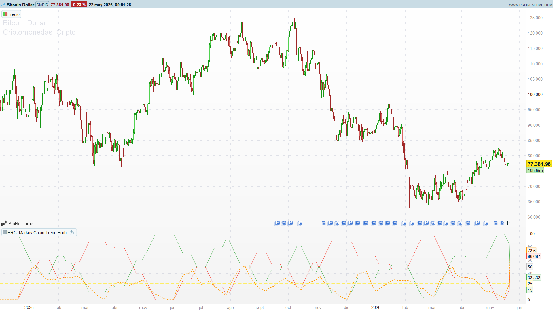
1. Green line — P(Up) %: empirical probability of UPTREND over the rolling window. When it sits above 70%, the recent regime has been dominantly bullish; when below 30%, dominantly bearish; around 50%, no clear regime bias.
2. Red line — P(Down) %: mirror of the green line (P(Down) = 100 − P(Up) by construction). Plotted explicitly because it makes regime balance visually obvious.
3. Orange dotted line — Brier Score %: calibration of the recent predictions. Below 15 (green reference line) the model is calibrated as “excellent”. Around 25 (yellow reference line) it is no better than random. Above 30 the predictions are unreliable — discount everything else on the panel until calibration recovers.
4. Reference lines: 50 (neutral split), 25 (random baseline for Brier), 15 (excellence threshold for Brier).

The most useful read is the gap between green and red combined with Brier below 15: a wide gap (e.g. P(Up) = 80%, P(Down) = 20%) with low Brier means the regime is both clear and the model has been tracking it accurately.

Practical Applications

1. Regime filter for trend-following systems. Only take long signals when P(Up) > 60% and Brier < 20%. The Brier gate keeps you out during transitional periods where the probability is high but unreliable.
2. Mean-reversion gate. Conversely, mean-reversion systems benefit from P(Up) ≈ P(Down) ≈ 50% (no regime) — the indicator can be used as a not-trending filter.
3. Confidence-weighted position sizing. The probability of the dominant state can scale position size: a 75% UPTREND probability with low Brier justifies a larger long exposure than a 55% probability with high Brier.
4. Diagnostic for the underlying chain. If P(Up→Up) and P(Down→Down) (computed internally) are both high, the market is in a strongly autocorrelated regime — favourable for trend-following. If they are both low, the market is fast-flipping — favourable for short-term mean reversion.

Indicator Configuration

| Parameter | Default | Description |
|-----------|---------|-------------|
| `lookbackPeriod` | 14 | Window in bars for price change |
| `atrThreshold` | 0.5 | Multiplier of ATR for the dead zone; higher = stickier regime |
| `historyLength` | 33 | Number of recent states kept for probability estimation |
| `atrLength` | 14 | ATR period |
| `brierLB` | 20 | Window of (prediction, outcome) pairs for Brier Score |

A higher atrThreshold produces fewer state changes, more regime persistence, and a higher P(Up→Up) / P(Down→Down). A larger historyLength makes the probabilities slower to adapt but more statistically reliable.

Implementation Notes

Translating this indicator to ProBuilder required several design choices worth documenting, as the Pine version makes heavy use of TradingView’s dynamic arrays and visual primitives that have no direct ProBuilder counterpart.

1. Dynamic arrays as fixed-slot FIFOs with shift. Pine’s array.unshift / array.pop pair (insert at the front, drop from the back) is replaced by a fixed-size ProBuilder array with a manual shift on each bar:

for k = historyLength - 1 downto 1 do
    $stateHist[k] = $stateHist[k - 1]
next
$stateHist[0] = currentState

The loop runs historyLength - 1 operations per bar. With historyLength = 33 this is trivial (~30 ops). A parallel stateCount counter tracks how many slots are valid during the warm-up period.

2. State machine with carry-over. ProBuilder’s IF/ELSIF chains do not implicitly retain a variable’s previous value. The “keep previous state” branch must be written explicitly:

if barindex < warmup then
    currentState = UPTREND
elsif atrNormChange > atrThreshold then
    currentState = UPTREND
elsif atrNormChange < 0 - atrThreshold then
    currentState = DOWNTREND
else
    currentState = currentState[1]
endif

Without the final else, the state would silently become undefined whenever the dead zone is hit, and the whole state machine would collapse.

3. Brier predictions stored one bar late to avoid data leakage. The prediction stored at bar t is probUp[1] — the value computed at the close of bar t-1, before the outcome of bar t was known. Pairing it with currentState of bar t gives an honest prediction/outcome pair.

$predHist[0] = probUp[1]
if currentState = UPTREND then
    $actHist[0] = 1
else
    $actHist[0] = 0
endif

4. Transition direction. The transition counter iterates pairs (slot[i+1], slot[i]) and interprets the older slot as the “from” state and the newer slot as the “to” state. This matches the standard chronological reading of a Markov transition: “given the state at time t, what is the probability of state at time t+1?”. The original Pine code computed the reverse direction; the ProBuilder port restores the chronological order so P(Up→Up) measures the canonical first-order transition probability.

5. What was lost from the original. Five elements of the Pine version have no clean ProBuilder equivalent and were dropped:

• The dashboard table (Current State, ATR Change, P(Up), P(Down), P(Up→Up) | P(Down→Down), Model Accuracy text). ProBuilder has no native tables. The information is still computed and visible in the panel as numeric series.
• The background colour based on the current state. ProBuilder indicators do not support bgcolor(). The panel uses three coloured series instead.
• The six predefined alerts. In ProRealTime, alerts are created from the UI directly on the returned series (right-click on the indicator line). No JSON payloads or alert messages are bundled with the indicator code.
• The colour and line-style inputs. ProBuilder requires literal arguments to style() (the line type and width cannot be variables). Colours are hardcoded for a sober, theme-neutral look. Edit the coloured(...) arguments directly if you want to recolour.
• The seven horizontal reference lines are reduced to three (50, 25, 15) — the most informative ones. The visual panel stays readable with three series and three guides; seven additional lines would have been noise.

Code

//----------------------------------------------
//PRC_Markov Chain Trend Probability
//version = 0
//22.05.26
//Iván González @ www.prorealcode.com
//Traducido de "Markov Chain Trend Probability" (PineScript v5)
//Autor original: Henrique Centieiro
//Sharing ProRealTime knowledge
//----------------------------------------------
// === Inputs ===
lookbackPeriod = 14    // n: ventana de cambio de precio
atrThreshold = 0.5     // X: umbral en multiplos de ATR
historyLength = 33     // historico de estados para probabilidades
atrLength = 14         // periodo del ATR
brierLB = 20           // ventana para Brier Score

// Constantes de estado
UPTREND = 1
DOWNTREND = -1
//----------------------------------------------
// === ATR y cambio normalizado ===
//----------------------------------------------
atrValue = averagetruerange[atrLength]
priceChange = close - close[lookbackPeriod]

if atrValue > 0 then
   atrNormChange = priceChange / atrValue
else
   atrNormChange = 0
endif
//----------------------------------------------
// === State machine UPTREND / DOWNTREND con carry-over ===
//----------------------------------------------
warmup = max(lookbackPeriod, atrLength)

if barindex < warmup then
   currentState = UPTREND
elsif atrNormChange > atrThreshold then
   currentState = UPTREND
elsif atrNormChange < 0 - atrThreshold then
   currentState = DOWNTREND
else
   currentState = currentState[1]
endif
//----------------------------------------------
// === Buffer FIFO de estados (slot[0] = mas reciente) ===
//----------------------------------------------
once stateCount = 0

for k = historyLength - 1 downto 1 do
   $stateHist[k] = $stateHist[k - 1]
next
$stateHist[0] = currentState

if stateCount < historyLength then
   stateCount = stateCount + 1
endif
//----------------------------------------------
// === Probabilidades de transicion ===
// (cronologicas: slot[i+1] = anterior, slot[i] = siguiente)
//----------------------------------------------
upToUp = 0
upTotal = 0
downToDown = 0
downTotal = 0

if stateCount >= 2 then
   for i = 0 to stateCount - 2 do
      fromState = $stateHist[i + 1]
      toState = $stateHist[i]
      
      if fromState = UPTREND then
         upTotal = upTotal + 1
         if toState = UPTREND then
            upToUp = upToUp + 1
         endif
      elsif fromState = DOWNTREND then
         downTotal = downTotal + 1
         if toState = DOWNTREND then
            downToDown = downToDown + 1
         endif
      endif
   next
endif

if upTotal > 0 then
   pUpToUp = upToUp / upTotal
else
   pUpToUp = 0
endif

if downTotal > 0 then
   pDownToDown = downToDown / downTotal
else
   pDownToDown = 0
endif
//----------------------------------------------
// === Probabilidades estacionarias ===
//----------------------------------------------
upCount = 0
if stateCount > 0 then
   for i = 0 to stateCount - 1 do
      if $stateHist[i] = UPTREND then
         upCount = upCount + 1
      endif
   next
   probUp = upCount / stateCount
   probDown = 1 - probUp
else
   probUp = 0
   probDown = 0
endif
//----------------------------------------------
// === Brier Score ===
// Prediccion en t-1 vs outcome observado en t
//----------------------------------------------
once brierCount = 0

if stateCount >= 2 then
   for k = brierLB - 1 downto 1 do
      $predHist[k] = $predHist[k - 1]
      $actHist[k] = $actHist[k - 1]
   next
   $predHist[0] = probUp[1]
   if currentState = UPTREND then
      $actHist[0] = 1
   else
      $actHist[0] = 0
   endif
   
   if brierCount < brierLB then
      brierCount = brierCount + 1
   endif
endif

if brierCount > 0 then
   sumSq = 0
   for i = 0 to brierCount - 1 do
      diff = $predHist[i] - $actHist[i]
      sumSq = sumSq + diff * diff
   next
   brierPct = sumSq / brierCount * 100
else
   brierPct = undefined
endif
//----------------------------------------------
// === Salidas (escala 0..100) ===
//----------------------------------------------
pUpPct = probUp * 100
pDnPct = probDown * 100

// Lineas horizontales de referencia
linMid = 50
linBaseline = 25
linExcel = 15

return pUpPct coloured(76, 175, 80, 255) as "P(Up) %", pDnPct coloured(244, 67, 54, 255) as "P(Down) %", brierPct coloured(255, 152, 0, 255) style(dottedline, 2) as "Brier Score %", linMid coloured(150, 150, 150, 150) style(dottedline2, 1) as "Neutral 50%", linBaseline coloured(255, 235, 59, 200) style(dottedline2, 1) as "Random Baseline 25%", linExcel coloured(76, 175, 80, 200) style(dottedline, 1) as "Excellent 15%"