

Indicators & Basic Functions (ProBuilder)
Introducing ProBuilder
ProBuilder is ProRealTime’s programming language. It is used to design custom technical indicators, trading strategies (ProBackTest) or custom scans (ProScreener). ProBackTest and ProScreener are the subject of individual manuals, due to their specific programming requirements.
This BASIC-type language is easy to use and offers a wide range of possibilities.
You will be able to build your own programs that use the quotations of any instrument included in the ProRealTime offer, starting from the basic elements:
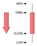
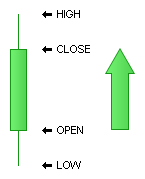
- the opening price of each bar: Open
- the closing price of each bar: Close
- the highest of each bar: High
- lowest of each bar: Low
- number of shares traded : Volume.
Bars, or candlesticks, are standard graphic representations of quotations received in real time. Of course, ProRealTime offers you the option of customizing the type of chart style, with views such as Renko, Kagi, Heikin-Ashi and others.
ProBuilder evaluates the data for each price bar from the oldest to the most recent, and executes the formula developed in the language to determine the value of the indicators on the bar in question.
Indicators developed in ProBuilder can be displayed on the price chart or in an individual chart, depending on the type of scale used.
In this document, you’ll gradually assimilate the commands needed to program in this language, thanks to a clear theoretical vision and concrete examples illustrating them.
At the end of this manual, you’ll find a glossary that will give you an overview of all ProBuilder commands, pre-coded indicators and other functions that will complement what you’ve learned during your reading.
Users who are more familiar with programming can skip ahead to Chapter II, or consult the glossary for a quick explanation of the function they are looking for.
For those less accustomed to programming, we recommend watching the video “Creating an indicator in ProBuilder” and reading the entire manual. The manual is highly practical and very directive, and we have no doubt that you’ll be able to master this language in no time.
If you have any further questions about how ProBuilder works, you can ask our ProRealTime community on the ProRealCode forum, where you’ll also find online documentation with numerous examples.
Wishing you every success and happy reading.
The ProRealTime team.
Chapter I: Fundamental concepts
Using ProBuilder
Indicator creation
The indicator programming area is available from the “Indicator” button in the bottom left-hand corner of every chart on your ProRealTime platform, or from the menu View > Indicators/Backtest.
You will then be taken to the indicator management window. You can :
- Display a predefined indicator.
- Create a custom indicator, which can then be applied to any value.
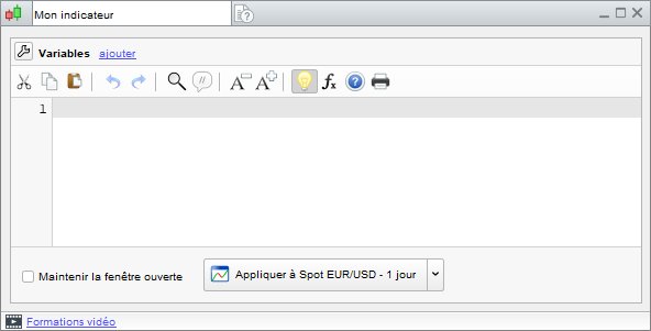
In the second case, click on “Create” to access the programming window.
You can then :
- Program an indicator directly into the code text box.
- Use the “Insert Function” help function ( icon), which opens a new window with a library of available functions, divided into eight categories, to assist you during programming.
Let’s take as an example the first characteristic element of ProBuilder indicators, i.e. the “RETURN” function (available in the “List of ProBuilder functions” section – see image below).
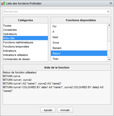
Select the word “RETURN” and click “Add”: the command will be added to the programming area.
![]() RETURN displays the result of your indicator
RETURN displays the result of your indicator
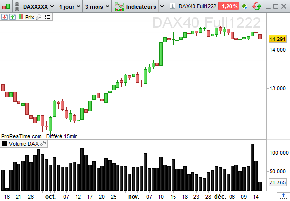
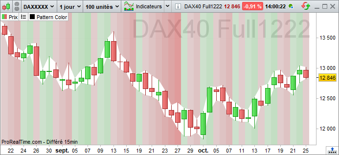
Let’s suppose we want to create an indicator displaying Volume. If you’ve already inserted the word RETURN, then simply go to “Insert function” again, click on “Constants” in the “Categories” section, then on the right-hand side, in the “Available functions” section, click on “Volume“. Finally, click on “Add”. Don’t forget to insert a space between each instruction.
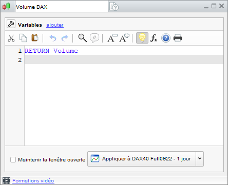
Before clicking on the “Apply to DAX” button, specify the name of your indicator at the top of the window: in this case, we’ve called it “DAX Volume”. Finally, click on “Apply to DAX” and you’ll see the chart with your indicator.
Code editor keyboard shortcuts
In ProRealTime version 12, the window for creating trading systems has several practical features that can be used via keyboard shortcuts:
- Select all (Ctrl+A): Selects all text in the code editor.
- Copy (Ctrl + C) : Copies selected text
- Paste (Ctrl + V) : Pastes copied text
- Undo (Ctrl + Z): Cancels the last action performed in the code editor
- Redo (Ctrl + Y): Redoes the last action performed in the code editor
- Find / Replace (Ctrl + F): Find text in code editor / Replace text in code editor
- Comment / Uncomment (Ctrl + R): Comment the selected code / Uncomment the selected code: the commented code will be preceded by “//” and colored gray. It will not be taken into account during code execution.
- Auto-completion (Ctrl+Space): Displays suggested instructions or keywords
For MAC users, the same keyboard shortcuts can be used. In this case, simply replace the “Ctrl” key with the “Command” key.
Most of these shortcuts can also be used via a right-click in the code editor.
Programming features of the ProBuilder language
Special features
The ProBuilder language allows you to manipulate many classic commands as well as more elaborate tools specific to technical analysis, giving you the ability to program indicators from the simplest to the most sophisticated.
The key principles to know about the ProBuilder language are :
- Variables do not need to be declared.
- Variables do not need to be typed.
- There’s no difference between upper and lower case.
- The same symbol is used for assignment and mathematical equality.
What does this mean?
- Declaring an X variable means indicating its existence. In ProBuilder, you can directly use X without having previously defined its existence. Let’s take an example by writing :
With declaration: Given a variable X, X is assigned the value 5
No declaration: X is assigned the value 5 (so X implicitly exists and is 5).
In ProBuilder, simply write: X=5
- Type a variable, i.e. define the nature of the variable: is it an integer (e.g.: 3; 8; 21; 643; …), a decimal number (e.g.: 1.76453534535…), a Boolean (TRUE, FALSE), …?
- In ProBuilder, you can write commands in either upper or lower case. For example, the set of commands IF / THEN / ELSE / ENDIF can be written as iF / tHeN / ELse / endIf.
- Assigning a value to a variable means giving it a value. To better understand the principle of assignment, think of a variable as an empty box waiting to be filled with something. The diagram below illustrates this principle with the value Volume assigned to variable X :
X Volume
See how the sentence reads from right to left: Volume is assigned to X.
Now, to write it in ProBuilder code, we simply replace the arrow with an = sign.
X = Volume
The same = symbol is used:
- For variable assignment (as in the previous example).
- As a mathematical comparison operator (1+ 1= 2 is equivalent to 2 = 1 + 1).
The execution model
Unlike conventional programming languages, which run once and then stop, ProBuilder runs once per candlestick, starting with the oldest candlestick.
When it reaches the candlestick under construction, the behavior changes according to the ProBuilder engine used (Indicator, Probacktest, ProOrder AutoTrading, ProScreener):
- In Indicator mode, the code is re-evaluated every tick.
- In ProBackest and ProOrder, the code is evaluated at candlestick closing.
- In ProScreener, the code is re-executed from the 1st candlestick as soon as the entire market has been scanned. This ensures that the ProScreener window is always up to date.
Variables
In conventional programming languages, variables contain a single value. In Probuilder, variables work differently. They store their values for each candlestick encountered. The history therefore grows as the code progresses over the historical candlesticks.
Each value in the history can be accessed at any time using the “[n]” operator to retrieve the value at n candlesticks in the past, relative to the current candlestick. It is also possible to retrieve the nth value in the history as follows: “[BarIndex-n]”.
- MaVariable[3]: Value of MaVariable 3 candlesticks before the current candlestick.
- MaVariable[BarIndex-3]: Value of MaVariable at the 3rd candlestick in the history
Although variables resemble lists in other programming languages, they function quite differently:
- It is impossible to modify the past: MyVariable[3] = 42 is not a valid instruction, the history can be read but not modified.
- Only the current candlestick value can be edited: MyVariable = 42
- A variable not edited in the current candlestick takes the value it had in the previous candlestick, as if the following instruction were inserted at the beginning of the code for each variable used in the code: MyVariable = MyVariable[1]
There are also array variables ($ MyArray[MyIndex] ), which will be discussed in detail later in this manual. Unlike conventional probuilder variables, arrays are not historized, so the following operation is invalid: “$ MyArray[MyIndex][3]”, which cannot read the value of$ MyArray[MyIndex] 3 candlesticks in the past.
![]() A good understanding of the execution model and the concept of historized variables is essential to use ProBuilder to its full potential!
A good understanding of the execution model and the concept of historized variables is essential to use ProBuilder to its full potential!
ProBuilder financial constants
Before starting to code your personal indicators, it is necessary to review the elements from which you will be able to build your code, such as opening and closing prices, volume, etc…
These are the “fundamentals” of technical analysis, and the essentials for coding indicators.
You can then combine them to highlight certain aspects of the information provided by the financial markets. They can be grouped into 5 categories:
Price and volume constants adapted to the time unit of the graph
These are the most commonly used “classic” constants. By default, they report the values of the current bar (whatever the time unit of the graph) and are presented as follows:
- Open: the opening price of the current bar.
- High: the highest price of the current bar.
- Low: the lowest price of the current bar.
- Close: the closing price of the current bar.
- Volume: the number of shares or lots traded on the current bar.
Example: Current bar range
a =  High
b =  Low
MyRange = a – b
RETURN MyRange
To call up the values of previous bars, simply add the number of bars to be considered (the number of bars from the current bar) in square brackets.
Let’s take the closing price constant as an example. The price is called up as follows:
Current bar close value : Close
Value for closing the bar preceding the current one : Close[1]
Close value of the nth bar preceding the current one: Close[n]
This rule applies to any constant. For example, the opening price of the 2nd bar preceding the current bar, will be called by : Open[2].
The value displayed will depend on the period displayed on the graph.
Daily price constants
Unlike constants adapted to the graph’s time unit, daily price constants refer to the day’s values, regardless of the period displayed on the graph.
Another difference with constants adapted to the time unit is that daily constants use parentheses to obtain their values on previous bars.
- DOpen(n) : opening price of the nth day prior to the current bar.
- DHigh(n): highest price of the nth day prior to the current bar.
- DLow(n): lowest price of the nth day prior to the current bar.
- DClose(n) : closing price of the nth day prior to the current bar.
Note: if “n” is 0, “n” refers to the current day. As maximum and minimum values are not yet definitive for n=0, we will obtain results that may change over the course of the day, depending on the minimum and maximum values reached.
![]() Brackets are used for constants adapted to the time unit, and brackets for daily constants. Close[3] DClose(3)
Brackets are used for constants adapted to the time unit, and brackets for daily constants. Close[3] DClose(3)
Time constants
Time is sometimes a neglected component of technical analysis. Yet traders are well aware of the importance of certain times of day, or certain dates of the year. It is therefore possible to limit the analysis of your indicator to specific times by using the following constants:
- Date: Date coded as YYYYMMDD indicating the closing date of each bar.
Time constants are treated by ProBuilder as integers. The Date constant, for example, must be presented as a single 8-digit number.
Let’s write the program :
RETURN Date
Suppose it’s July 4, 2020. The indicator from the above program will return the following result 20200704.
To read a date, simply read it as follows:
20200704 = 2020 years 07 months and 04 days.
Note that when writing a date in YYYYMMDD format, MM must be between 1 and 12 and DD must be between 1 and 31.
- Time: HourMinuteSecond coded as HHMMSS indicating the closing time of each bar.
For example:
RETURN Time
We obtain a curve linking all the closing times of each bar:
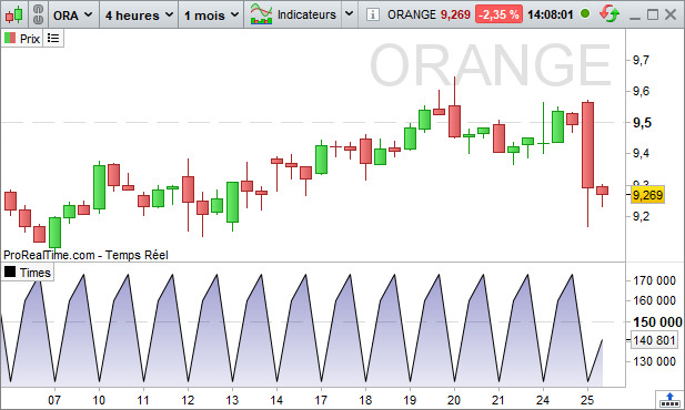
To read an hour, simply read as follows:
160000 = 16 hours 00 minutes and 00 seconds.
Note that when writing a time in HHMMSS format, HH must be between 0 and 23, MM must be between 0 and 59 and SS must also be between 0 and 59.
It is possible to combine Time and Date in the same indicator to restrict the result to a specific time. In the following example, we want to limit our indicator to the first of October 2008 at 9:00 and 1 sec.
a = (Date =  20081001)
b = (Time =  090001)
RETURN (a AND b)
The following constants work in the same way:
- Timestamp: UNIX date and time (number of seconds since January 1st 1970) of each bar closure.
- Second: Second of closure of each bar (between 0 and 59).
- Minute: Minute of closure of each bar (between 0 and 59).
- Hour: Closing time for each bar (between 0 and 23).
- Day: Day of the month in which each bar closes (between 1 and 28 or 29 or 30 or 31).
- Month: Month in which each bar closes (between 1 and 12).
- Year: Year of closure of each bar.
- DayOfWeek: Day of the week at the close of each bar (0=Sunday,1=Monday, 2=Tuesday, 3=Wednesday, 4=Thursday, 5=Friday,6=Saturday).
There is also an Open derivative:
- OpenTimestamp: UNIX date and time when each bar was opened.
- OpenSecond: Second of opening of each bar (between 0 and 59).
- OpenMinute: Minute of opening of each bar (between 0 and 59).
- OpenHour: Opening time for each bar (between 0 and 23).
- OpenDay: Day of the month each bar opens (between 1 and 28 or 29 or 30 or 31).
- OpenMonth: Month each bar opens (between 1 and 12).
- OpenYear: Year each bar was opened.
- OpenDayOfWeek: Day of the week when each bar opens (0=Sunday,1=Monday, 2=Tuesday, 3=Wednesday, 4=Thursday, 5=Friday,6=Saturday).
- OpenTime: HourMinuteSecond encoded as HHMMSS indicating the opening time of each bar.
- OpenDate: Date (YYYYMMDD) on which the current bar was opened.
Example of the use of these constants :
a = (Hour >  17)
b = (Day =  30)
RETURN (a AND b)- CurrentHour: Current time (market time).
- CurrentMinute: Current (market) minute.
- CurrentMonth: Current month (market month).
- CurrentSecond: Current (market) second.
- CurrentTime: Current time (market time).
- CurrentYear: Current year (market year).
- CurrentDayOfWeek: Day of the current week according to market time zone.
The difference between the Current constants proposed above and those without Current seen previously is precisely the “Current” aspect.
The following image illustrates this difference when applied to CurrentTime and Time constants. For simplicity’s sake, Current constants ignore the time axis and consider only the value displayed in the white box.
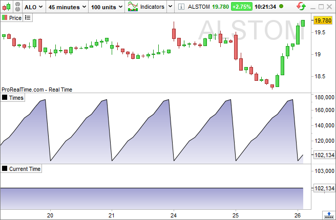
![]() Time indicates the closing time of each bar. CurrentTime indicates market time
Time indicates the closing time of each bar. CurrentTime indicates market time
If you wish to set your indicators in relation to counters (number of days elapsed, number of bars, etc.), the Days, BarIndex and IntradayBarIndex constants are available.
- Days: Day counter since 1900.
This constant is useful when you want to know the number of days that have elapsed, especially when working in quantitative views, such as (x)Tick or (x)Volumes.
The following example shows the transition from one day of quotations to the next, when you’re in one of these views.
RETURN Days
(Be careful not to confuse the two constants “Day” and “Days“).
- BarIndex: Bar counter since start of displayed history.
The counter starts from the leftmost bar in the loaded history and counts all bars up to and including the rightmost one. The first (leftmost) bar displayed is considered to be bar 0. BarIndex is usually used in conjunction with the IF instruction described later in this manual.
- IntradayBarIndex: Intraday bar counter.
The counter displays the number of bars since the start of the day and is reset to zero at the beginning of each day. The first bar in the counter is considered bar 0.
Let’s compare the two constants by creating two separate indicators:
RETURN BarIndex
and
RETURN IntradayBarIndex
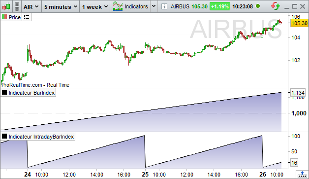
IntradayBarIndex resets the bar counter at the start of each day.
Price-derived constants
- Range: difference between High and Low.
- TypicalPrice: average between High, Low and Close.
- WeightedClose: weighted average of High (weight 1), Low (weight 1) and Close (weight 2).
- MedianPrice: the average between High and Low.
- TotalPrice: the average of Open, High, Low and Close.
Range represents the volatility of the current bar.
WeightedClose emphasizes the importance of the closing price.
The TypicalPrice and TotalPrice constants better reflect current intra-bar market psychology, as they take into account three and four price levels reached during this candlestick.
The MedianPrice represents the average price of the extremums.
Range in % :
MyRange =  Range
Calculation = (MyRange / MyRange[1] – 1) * 100
RETURN Calculation
The indefinite constant
Undefined allows you to tell the indicator not to display a result for certain variables (by default, all unassigned variables are set to zero).
- Undefined: undefined data (equivalent to an empty box).
You can find a sample application later in the manual.
Use of pre-existing indicators
So far, we’ve taken a look at the possibilities offered by Probuilder in terms of constants and their behavior when accessing past bars. The same behavior applies to the operation of pre-existing indicators (and later we’ll see that those you program will operate on the same principle).
ProBuilder indicators consist of three elements whose syntax is :
FunctionName [calculated on n bars] (on such and such a variable)
When you use the “Insert Function” button to search for a ProBuilder function, default values are set for the period and for the price or indicator argument. Example for a 20-period moving average:
Average[20](Close)
We can, of course, modify them according to our preferences; for example, we can replace the 20 bars defined by default by any other number of bars (e.g. Average[10], Average[15],Average[30],…,Average[n]). Similarly, you can change the price argument or indicator, such as the RSI (Relative Strength Index). We’ll get, for example :
Average[20](RSI[5](Close))
We thus calculate the 20-period moving average of an RSI calculated over 5 periods.
Let’s look at a few examples of the behavior of pre-existing indicators:
Program calculating the exponential moving average over 20 candles applied to the closing price: RETURN ExponentialAverage[20](Close)
Calculation of a weighted moving average over 20 bars applied to the typical price: RETURN WeightedAverage[20](TypicalPrice)
Calculation of a Wilder-smoothed moving average over 100 bars applied to Volume: RETURN WilderAverage[100](Volume)
Calculation of MACD (histogram) on closing price.
The MACD line is constructed as the difference between the 12-period exponential moving average minus the 26-period exponential moving average. A 9-period exponential moving average is then applied to the difference to obtain the Signal line. The MACD histogram is then calculated as the difference between the MACD line and the Signal line.
// MACD line calculation
MACDLine =  ExponentialAverage[12](Close) – ExponentialAverage[26](Close)
// MACD signal line calculation
LineSignal =  ExponentialAverage[9](LineMACD)
// Calculation of the difference between the MACD line and its Signal
MACDHistogram =  LineMACD – LineSignal
RETURN MACDHistogram
Two-parameter averaging
You can also set the average function with a second parameter. We obtain the following formula:
Average[No. of periods, Type of average]
The Average type parameter designates the type of average to be used. There are 9 of them, indexed from 0 to 8:
- 0 – Simple Moving Average (SMA)
- 1 – Exponential Moving Average (EMA)
- 2 – Weighted Moving Average (WMA)
- 3 – Wilder’s Moving Average
- 4 – Triangular Moving Average
- 5 – End Point Moving Average
- 6 – Time Series Moving Average
- 7 – Hull Moving Average
- 8 – ZeroLag Moving Average
Calculating Ichimoku lines
As the Ichimoku indicator has many lines representing it, some of these lines have been introduced into the ProBuilder language to enable you to make full use of its potential.
The lines are as follows:
- SenkouSpanA[TenkanPeriod,KijunPeriod,Senkou-SpanBPeriod]
- TenkanSen[TenkanPeriod,KijunPeriod,Senkou-SpanBPeriod]
- KijunSen[TenkanPeriod,KijunPeriod,Senkou-SpanBPeriod]
- SenkouSpanB[TenkanPeriod,KijunPeriod,Senkou-SpanBPeriod]
With the usual Ichimoku parameters for each line:
- TenkanPeriod: alert line, (high point + low point)/2 over the last n periods
- KijunPeriod: signal line, (high point + low point)/2 over the last n periods
- Senkou-SpanBPeriod: long-term average point projection, (high point + low point)/2 over the last n periods
Calculation of PRT Bands
PRT Bands is a visual indicator that simplifies trend detection and monitoring. It is exclusive to the ProRealTime platform.
It can help you :
- detect a trend reversal
- identify and follow an uptrend
- measure trend intensity
- find potential entry and exit points
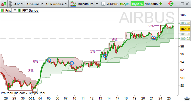
Here are the different PRT Bands data available in the ProBuilder language:
- PRTBANDSUP: returns the value of the top line of the indicator
- PRTBANDSDOWN: returns the value of the bottom line of the indicator
- PRTBANDSSHORTTERM: returns the value of the indicator’s short-term (thick) line
- PRTBANDSMEDIUMTERM: returns the value of the indicator’s medium-term (thin) line
Find out more about the PRT Bands indicator
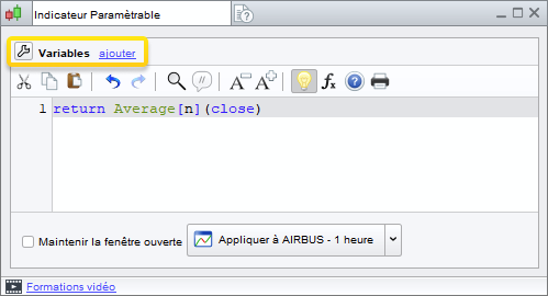
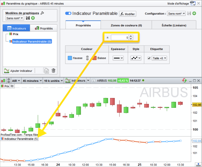
Adding configurable variables
When coding an indicator, a number of constants are introduced. The parameterizable variables option, at top left, lets you assign a default value to an undefined variable, and then act on the value of this variable from the indicator parameters interface.
The advantage lies in the possibility of modifying the indicator parameters without modifying the code.
For example, let’s calculate a moving average of period 20 :
RETURN Average[20](Close)
To modify the number of calculation periods directly from the interface, replace 20 with an ‘n’ variable:
RETURN Average[n](Close)
Then click on “Add” next to “Variables”, and the “Variables definition” window will appear.
Enter the name of your variable, here “n” and click on “Add”, you will then be able to enter a Type and a Default Value, Fill in as follows:
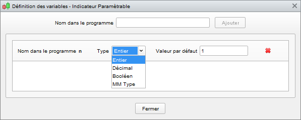
Then click on “Close”.
In the Indicator Properties window, you’ll get a new parameter, which will allow you to act on the period of the moving average:
List of types available for parameterizable variables :
- Integer: integer between -2,000,000,000 and 2,000,000,000 (e.g. 450)
- Decimal: decimal number accurate to 5 significant digits (e.g. 1.03247)
- Boolean: True (1) or False (0)
- Moving average type: defines the value of the second parameter for calculating the moving average of the Average indicator (see above).
Of course, it is possible to create several variables, allowing you to modify several parameters at the same time.
Chapter II: ProBuilder functions and instructions
Control structures
Conditional instruction IF
The IF statement is used to select conditional actions, i.e. to subordinate a result to the verification of one or more defined conditions.
The structure is made up of IF, THEN, ELSE, ELSIF and ENDIF elements, which can be combined according to the complexity of the conditions we want to define. Let’s take a look at how they work.
One condition, one result (IF THEN ENDIF)
We can search for a condition and define an action if the condition is met. On the other hand, if the condition is not met, nothing happens (default 0).
In the example, if the last price is higher than the period 20 MM, then the value 1 is displayed.
Result = 0 // Result equals 0.
IF Close> Average[20](Close) THEN // If the closing price is > the 20-period moving average
Result = 1 // THEN Result will equal 1
ENDIF // END OF CONDITION
RETURN Result![]() RETURN must always be followed by the storage variable used (in the example, Result) if the result of the condition is to be displayed.
RETURN must always be followed by the storage variable used (in the example, Result) if the result of the condition is to be displayed.
One condition, two results (IF THEN ELSE ENDIF)
We can also choose to define a result in case the condition is not verified. Let’s take the previous example: if the last price is higher than the MM for period 20, we display the value 1.
Otherwise, -1 is displayed.
IF Close> Average[20](Close) THEN
Result = 1
ELSE
Result = -1
ENDIF
RETURN Result
NB: We’ve just created a binary indicator. To find out more, see the section on binary and ternary indicators later in this manual.
Nested conditions
It is possible to create sub-conditions following the validation of a main condition, i.e. conditions that must be verified one after the other (in order of appearance). To do this, simply nest the IFs, taking care to insert as many ENDIFs as IFs. Let’s take a look at the example :
Double conditions on moving averages :
IF (Average[12](Close) – Average[20](Close) > 0) THEN
IF ExponentialAverage[12](Close) – ExponentialAverage[20](Close) > 0 THEN
Result = 1
ELSE
Result = -1
ENDIF
ENDIF
RETURN Result
Multiple conditions (IF THEN ELSIF ELSE ENDIF)
It is possible to define several results, each associated with a specific condition. The indicator therefore reports several states: if Condition1 is verified, Action 1 is activated; otherwise, if Condition 2 is verified, Action 2 is activated…if no condition is verified, Action n is activated.
Syntactically, this structure uses the statements: IF, THEN, ELSIF, THEN … ELSE, ENDIF.
It is written as follows:
IF (Condition1) THEN
(Action1)
ELSIF (Condition2) THEN
(Action2)
ELSIF (Condition3) THEN
(Action3)
…
ELSE
(Action n)
ENDIF
It is possible to replace ELSIFs with ELSE IFs, but this is more cumbersome. You would then have to end the series with as many ENDIFs as IFs written. If you wish to nest multiple conditions in your program, you are advised to use ELSIF rather than ELSE IF.
Example: detecting bullish and bearish trends
This indicator will return 1 if a bullish advance is detected, -1 if a bearish advance is detected and 0 the rest of the time.
| // Description of a bullish trend Condition1 = Close[1] < Open[1] Condition2 = Open < Close[1] Condition3 = Close > Open[1] Condition4 = Open < Close |
 |
| // Description of a bearish move Condition5 = Close[1] > Open[1] Condition6 = Close < Open Condition7 = Open > Close[1] Condition8 = Close < Open[1] |
 |
IF Condition1 AND Condition2 AND Condition3 AND Condition4 THEN
a = 1
ELSIF Condition5 AND Condition6 AND Condition7 AND Condition8 THEN
a = -1
ELSE
a = 0
ENDIF
RETURN a
Example: Demarks pivot Resistance
IF DClose(1) > DOpen(1) THEN
Phigh =  DHigh(1) + (DClose(1) – DLow(1)) / 2
Plow = (DClose(1) + DLow(1)) / 2
ELSIF DClose(1) < DOpen(1) THEN
Phigh = (DHigh(1) + DClose(1)) / 2
Plow =  DLow(1) – (DHigh(1) – DClose(1)) / 2
ELSE
Phigh =  DClose(1) + (DHigh(1) – DLow(1)) / 2
Plow =  DClose(1) – (DHigh(1) – DLow(1)) / 2
ENDIF
RETURN Phigh , Plow
Example: BarIndex
In Chapter I of this manual, BarIndex was introduced as a counter for the number of bars since the start of the displayed history. BarIndex is often used in conjunction with IF. For example, if we want to know whether our graph contains fewer or more than 23 bars, we’ll write :
IF BarIndex<= 23 THEN
a = 0
ELSIF BarIndex> 23 THEN
a = 1
ENDIF
RETURN a
Iterative loop FOR
The FOR loop is used when you want to go through a finite, ordered list of numbers one by one (1,2,3,…,6,7 or 7,6,…,3,2,1).
The structure consists of the keywords FOR, TO, DOWNTO, DO, NEXT. The use of TO or DOWNTO varies according to whether the elements are called in ascending or descending order. It’s important to note that what lies between FOR and DO are the limits of the interval to be scanned.
Increasing advance (FOR, TO, DO, NEXT)
FOR Variable = SeriesStartValue TO SeriesEndValue DO
(Action)
NEXT
Example: smoothing a 12-period moving average (MM12)
We’ll create a storage variable (Result) which will sum each moving average, one by one, for periods 11, 12 and 13.
Result = 0
FOR Variable = 11 TO 13 DO
Result =  Result +  Average[Variable](Close
NEXT
// Average the moving averages by dividing Result by 3 and storing the result in AverageResult.
AverageResult =  Result / 3
RETURN AverageResult
Let’s visualize what happens step by step:
Mathematically, we want to average the arithmetic moving averages for periods 11, 12 and 13.
Variable will therefore successively take the values 11, 12 then 13
Result = 0
Variable = 11
Result receives the value of the previous Result + MM11 i.e.: (0) + MM11 = (0 + MM11)
The NEXT instruction takes us to the next counter value
Variable = 12
Result receives the value of the previous Result + MM12 i.e.: (0 + MM11) + MM12 = (0 + MM11 + MM12)
The NEXT instruction takes us to the next counter value
Variable = 13
Result receives the value of the previous Result + MM13 i.e.: (0 + MM11 + MM12) + MM13 = (0 + MM11 + MM12 + MM13)
Value 13 is the last counter value.
NEXT closes the FOR loop, as there is no next value.
Result is displayed
This code simply means that Variable will first take the value at the start of the series, then Variable will take the next value (the previous one + 1) and so on until Variable exceeds or equals the value at the end of the series. Then the loop ends.
Example: Average of the last 5 high bars
SUMhigh = 0
IF BarIndex < 5 THEN // If there are no more than 5 periods in the history
MMhigh = Undefined // So we set MMhigh to the default value of “nothing”.
ELSE // Otherwise
FOR i = 0 TO 4 DO // For values between 0 and 4
SUMhigh = High[i] + SUMhigh // We sum the last 5 values of the highest
NEXT
ENDIF
MMhigh = SUMhigh / 5 // We average this sum by 5 and assign it to MMhigh
RETURN MMhigh // MMhigh is displayed
Descending advance (FOR, DOWNTO, DO, NEXT)
In contrast, the instructions FOR, DOWNTO, DO, NEXT are used for decreasing advancement.
It is written as follows:
FOR Variable = SeriesEndValue DOWNTO SeriesBeginValue DO
(Action)
NEXT
Let’s take the example of the moving average over the last 5 highest price bars:
Note that we’ve just inverted the limits of the swept interval.
SUMhigh = 0
IF BarIndex <  5 THEN
MMhigh =  Undefined
ELSE
FOR i = 4 DOWNTO 0 DO
SUMhigh =  High[i] + SUMhigh
NEXT
ENDIF
MMhigh =  SUMhigh / 5
RETURN Mmhigh
WHILE conditional loop
The WHILE loop is used to apply actions as long as a condition remains valid. You’ll see that this loop has a lot in common with the simple IF/THEN/ENDIF conditional statement.
Syntactically, this structure uses the following instructions: WHILE,(DO optional), WEND
The structure is written as follows:
WHILE (Condition) DO
(Action 1)
…
(Action n)
WEND
This code highlights the number of bars separating the current candlestick from a higher previous candlestick, up to a limit of 30 periods.
i = 1
WHILE high >  high[i] AND i < 30 DO
i = i + 1
WEND
RETURN i
Example: indicator calculating the number of consecutive upward periods
Increase = (Close >  Close[1])
Count = 0
WHILE Increase[Count] DO
Count = Count + 1
WEND
RETURN Count
General note on the WHILE conditional statement :
In the same way as for IF, the program will automatically assign the value 0 when the validation condition is unknown.
Let’s take an example:
Count = 0
WHILE i <> 11 DO
i = i + 1
Count = Count + 1
WEND
RETURN Count
In the above code, as the variable i is not defined, it will automatically take the value 0 during the first loop and this from the first candlestick.
The loop will use its resources to set the variable i to the default value of 0. Count will be well processed, hence the 0 return value, as its value is re-initialized at the start of each candlestick, and i will be greater than 11 at the end of the first candlestick, preventing entry into the loop for the next candlestick. Setting i from the outset will produce very different results:
i = 0
Count = 0
WHILE i <> 11 DO
i = i + 1
Count = Count + 1
WEND
RETURN Count
In this code, i is initialized to 0 at the start of each candlestick, so we pass through the loop each time and have 11 and 11 as return values for i and count.
BREAK
The BREAK instruction can be used to force an exit from a WHILE or FOR loop. Combinations with the IF command are possible, whether in a WHILE loop or a FOR loop.
Break with WHILE
When we want to get out of a WHILE conditional loop, i.e. we don’t expect to find a situation that doesn’t satisfy the looping condition, we use BREAK according to the following structure:
WHILE (Condition) DO
(Action)
IF (ConditionBreak) THEN
BREAK
ENDIF
WEND
Using BREAK in a WHILE loop is only useful if you want to test an additional condition whose value can only be known in the body of the WHILE loop. Take, for example, a stochastic based on an oscillator which is only calculated in an uptrend:
line = 0
Increase = (Close – Close[1]) > 0
i = 0
WHILE Increase[i] DO
i = i + 1
// If high – low, exit the loop to avoid division by zero.
IF (High-Low) = 0 THEN
BREAK
ENDIF
osc = (Close – Low) / (High – Low)
line =  AVERAGE[i](osc)
WEND
RETURN line
Break with FOR
When you want to exit a FOR iterative loop without arriving at the last (or first) value in the series, use BREAK according to the following structure:
FOR Variable = SeriesStartValue TO SeriesEndValue DO
(Action)
BREAK
NEXT
For example, let’s take an indicator that cumulates the number of consecutive volume increases over the last 19 bars. This indicator will return zero if volume is bearish.
Indicator = 0
FOR i = 0 TO 19 DO
IF (Volume[i] > Volume[i + 1]) THEN
Indicator = Indicator + 1
ELSE
BREAK
ENDIF
NEXT
RETURN Indicator
In this code, if BREAK had not been used, the loop would have continued to 19 (the last element in the series), even though the volume condition is invalid.
With BREAK, on the other hand, as soon as the condition is no longer validated, it returns the result.
CONTINUE
The CONTINUE instruction is used to finish the current iteration of a WHILE or FOR loop. It is often used in conjunction with BREAK, to give the command either to exit the loop (BREAK) or to remain in it (CONTINUE).
Continue with WHILE
Let’s create a program to accumulate the number of candlesticks with a higher close and a lower open than the previous day. If the condition is not met, the counter will return to zero.
Increase =  Close> Close[1]
condition = Open> Open[1]
Count = 0
WHILE condition[Count] DO
IF Increase[Count] THEN
Count = Count + 1
CONTINUE
ENDIF
BREAK
WEND
RETURN Count
Thanks to CONTINUE, when the IF condition is verified, you don’t exit the WHILE loop, thus accumulating the number of candlesticks verifying this condition. Without the CONTINUE instruction, the program would exit the loop, whether or not the IF condition is verified. It would therefore be impossible to accumulate condition occurrences, and the result would be binary (1,0).
Continue with FOR
Let’s create a program to accumulate the number of candlesticks with a higher close than the previous day. If the condition is not met, the counter will return to zero.
Increase = Close> Close[1]
Count = 0
FOR i = 1 TO BarIndex DO
IF Increase[Count] THEN
Count = Count + 1
CONTINUE
ENDIF
BREAK
NEXT
RETURN Count
FOR allows you to test the condition on the entire available history. Thanks to CONTINUE, when the IF condition is verified, we don’t exit the FOR loop and continue with the next i value. This accumulates the number of figures verifying the condition.
Without the CONTINUE instruction, the program would exit the loop, whether or not the IF condition is verified.
The number of figures appearing could therefore not be accumulated, and the result would be binary (1,0).
![]() It’s important to make sure you always have a valid exit condition for FOR and WHILE loops to ensure your code works properly.
It’s important to make sure you always have a valid exit condition for FOR and WHILE loops to ensure your code works properly.
ONCE
The ONCE instruction is used to declare a variable “only once“.
Knowing that for any program, the language will read the code as many times as there are bars on the graph before returning a result, you should remember that ONCE :
- It is processed by the program only once, including proofreading.
- When the language rereads the code, it retains the values calculated during the previous reading.
To fully understand how this command works, you need to understand how the language reads the code; hence the usefulness of the following example.
Here are two programs that return 0 and 15 respectively, the only difference being the addition of the ONCE command:
| Program 1 | Program 2 | ||
| 1
2 3 4 5 6 7 |
Count = 0
i = 0 IF i <= 5 THEN Count = Count + i i = i + 1 ENDIF RETURN Count |
1
2 3 4 5 6 7 |
ONCE Count = 0
ONCE i = 0 IF i <= 5 THEN Count = Count + i i = i + 1 ENDIF RETURN Count |
Let’s see how the language has read the codes.
Program 1 :
The language reads L1 (Count = 0; i = 0), then L2, L3, L4, L5 and L6 (Count = 0; i = 1), returns to L1 and reads everything again in exactly the same way. The result displayed is 0 (zero), as after the first reading.
Program 2 :
The language will read L1 (Count = 0; i = 0), then L2, L3, L4, L5, L6 (Count = 0; i = 1); when it reaches the RETURN line, it starts the loop again from L3 (lines with ONCE are only processed the first time), L4, L5, L6 (Count = 1; i = 2), then returns again (Count = 3; i = 3) and so on up to (Count = 15; i = 6). When this result is reached, the IF instruction is no longer processed, as the condition is no longer valid; only L7 remains to be read. Hence the result: 15.
Mathematical functions
Common unary and binary functions
Let’s turn now to mathematical functions.
Note that a and b are examples of decimal arguments. They can be replaced by any variable in your program.
- MIN(a, b): calculates the minimum of a and b
- MAX(a, b): calculates the maximum of a and b
- ROUND(a, n): calculates a rounded to unity with a precision of n decimal places
- ABS(a): calculates the absolute value of a
- SGN(a): gives the sign of a (1 for positive, -1 for negative, 0 if zero)
- SQUARE(a): calculates the square of a
- SQRT(a): calculates the square root of a
- LOG(a): calculates the natural logarithm of a
- POW(a,b): calculates a to the power b
- EXP(a): calculates the exponential of a
- COS(a) / SIN(a) / TAN(a): calculates the cosine/sinus/tangent of a (in degrees)
- ACOS(a) / ASIN(a) / ATAN(a): calculates the arc-cosine/arc-sine/arc-tangent (in degrees) of a
- FLOOR(a, n): returns the largest integer less than a with a precision of n
- CEIL(a, n): returns the smallest integer greater than a with a precision of n
- RANDOM(a,b): generates a random integer between a and b (inclusive)
For example, let’s take the mathematical normal law, which is interesting because it uses squaring, square-root and exponential:
// Normal law applied to x = 10, Standard deviation = 6 and Expectation = 8
// As an optimized variable :
Standard deviation = 6
Esperance = 8
x = 10
Indicator = EXP( –  (1/2)*(SQUARE(x-Esperance)/Ecarttype))/(Ecarttype*SQRT(2/3.1415))
RETURN Indicator
Common mathematical operators
- a < b: a is strictly less than b
- a <= b or a =< b: a is less than or equal to b
- a > b: a is strictly greater than b
- a >= b or a => b: a is greater than or equal to b
- a = b: a equals b (or a receives the value b)
- a <> b: a is different from b
Graphical comparison functions
- a CROSSES OVER b: a crosses b on the upside
- a CROSSES UNDER b: a crosses b on the downside
Summation functions
- cumsum: Calculates the sum of all bars on the graph
The syntax for using cumsum is :
cumsum(price or indicator)
- summation: Calculates the sum over a specified number of bars
The sum is calculated from the most recent bar (from right to left).
The syntax for using summation is :
summation[number of bars](price or indicator)
Statistics functions
The syntax for using these functions is the same as for indicators and the Summation function, i.e. :
lowest[number of bars](price or indicator)
- Lowest: gives the lowest value over the defined period
- Highest: gives the highest value over the defined period
- STD: gives the standard deviation of a value for a defined period
- STE: gives the error deviation on a value for a defined period
Logic operators
Likewise, as with any computer language, you need logical operators to create relevant indicators. Below you’ll find ProBuilder’s 4 logical operators:
- NOT a : logical NO
- a OR b: logical OR
- a AND b: logical AND
- a XOR b: exclusive OR (a OR b but not a AND b)
Calculation of trend indicator: On Balance Volume (OBV) :
IF NOT((Close> Close[1]) OR (Close= Close[1])) THEN
MyOBV= MyOBV – Volume
ELSE
MyOBV= MyOBV+ Volume
ENDIF
RETURN MyOBV
Keywords ProBuilder
- RETURN: displays the result of your indicator
- CALL: calls a function previously created by the user
- AS: names the different results displayed
- COLOURED: colors the displayed trace with a color to be defined
RETURN
In the first chapter, we saw the importance of the RETURN instruction. It has special properties that you need to be aware of to avoid certain programming errors.
For correct use when writing a program, RETURN is used :
- Once and for all
- On the last line of code
- Optionally with other functions such as AS, COLOURED and STYLE
- To display several results, write RETURN followed by the results to be displayed, separated by a comma (example: RETURN a,b).
Comments
// or /**/ allow you to place comments in the code. Their main purpose is to remind you how a function you’ve coded works. These comments will be read but not processed by the code. Let’s illustrate the idea with the following example:
// this program returns the period 20 arithmetic moving average of the closing price
RETURN Average[20](Close)![]() Do not use special characters (e.g. é,ù,ç,ê…) in ProBuilder (this does not apply to comments).
Do not use special characters (e.g. é,ù,ç,ê…) in ProBuilder (this does not apply to comments).
CustomClose
CustomClose is a variable that displays the constants Close, Open, High, Low and other values, which can be selected in the indicator properties window.
Its syntax is the same as that of price constants, which adapt to the graph view:
CustomClose[n]
Let’s take a simple example:
RETURN CustomClose[2]
By clicking on “Configure” from the price label in the top left-hand corner of the chart, you’ll see that it’s possible to configure the prices used for calculation.
CALCULATEONLASTBARS
CALCULATEONLASTBARS: This parameter increases the speed at which an indicator is calculated by defining the number of bars that can be used to calculate the indicator. The display will start with the most recent bar.
Example: DEFPARAM CALCULATEONLASTBARS = 200
Please note: the DEFPARAM instruction be used at the beginning of the code.
CALL
CALL allows you to call up a custom indicator already present on your platform.
The quickest way is to select the indicator to be used directly from the “User indicators” category (in the “Insert function” menu).
Let’s say you’ve coded the MACD histogram indicator as HistoMACD.
Select your indicator and click on “Add” and in the programming area will appear :
myHistoMACD = CALL “HistoMACD”
The software itself has renamed your old “HistoMACD” indicator to “myHistoMACD”.
This means that for the rest of your program, if you want to use this HistoMACD indicator, you’ll have to call it “myHistoMACD”.
An example is when several variables are returned by your CALL :
myExponentialMovingAverage, mySimpleMovingAverage = CALL “Averages”
AS
The AS keyword is used to name the displayed result. This instruction is used with RETURN according to the following structure:
RETURN Result1 AS “Curve Name1”, Result2 AS “Curve Name2”, …
This keyword makes it easier to identify the components of the indicator created.
Example:
a = ExponentialAverage[200](Close)
b = WeightedAverage[200](Close)
c = Average[200](Close)
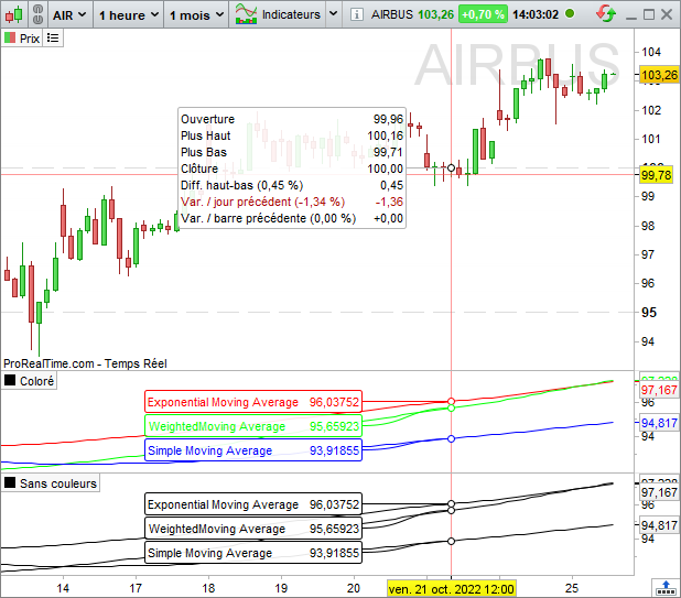
RETURN a AS “Exponential Average”, b AS “Weighted Average”, c AS “Arithmetic Average”.COLOURED
COLOURED is used after the RETURN command to color the displayed value with a certain color, defined according to the RGB standard (Red, Green, Blue) or using pre-defined colors.
The 140 pre-defined colors can be found in the following documentation:
W3 School : HTML Color Names
The main colors of the RGB standard and their pre-defined HTML names are given below:
| COLOR | RGB VALUE (between 0 and 255) (RED, GREEN, BLUE) |
HTML Color Name |
| ⏹︎ | (0, 0, 0) | black |
| (255, 255, 255) | white | |
| ⏹︎ | (255, 0, 0) | red |
| ⏹︎ | (0, 255, 0) | green |
| ⏹︎ | (0, 0, 255) | blue |
| ⏹︎ | (255, 255, 0) | yellow |
| ⏹︎ | (0, 255, 255) | cyan |
| ⏹︎ | (255, 0, 255) | magenta |
The syntax for using the COLOURED command is as follows:
RETURN Indicator COLOURED(RedValue, GreenValue, BlueValue)
Or else
RETURN Indicator COLOURED(“cyan“)
Optionally, you can control the opacity of your curve with the alpha parameter (ranging from 0 to 255):
RETURN Indicator COLOURED(RedValue, GreenValue, BlueValue, AlphaValue)
The AS command can be combined with the COLOURED(., ., .) command:
RETURN Indicator COLOURED(RedValue, GreenValue, BlueValue) AS “Name Of My Curve”
Let’s go back to the previous example and insert COLOURED in the “RETURN” line.
a = ExponentialAverage[200](Close)
b = WeightedAverage[200](Close)
c = Average[200](Close)
RETURN a COLOURED(“red”) AS “Exponential Moving Average”, b COLOURED(“green”) AS “WeightedMoving Average”, c COLOURED(“blue”) AS “Simple Moving Average”
The image shows the color customization in the result.
Drawing commands
These commands let you draw objects on the graphics, as well as customize your candles, the bars of your graphics and the colors of all these elements.
For each instruction below, the color can be defined in a similar way to the color of your curve (COLOURED instruction above) with either a predefined color (HTML Color Names) in quotation marks, or a triplet (R,G,B) to which you can apply an alpha opacity parameter: (“HTML Color Names”,alpha) or (R,G,B,alpha).
- BACKGROUNDCOLOR(R,G,B,a): Allows you to color the background of graphs or specific bars (such as odd or even days). The colored area starts midway between the previous and next bars.
Example: BACKGROUNDCOLOR(0, 127, 255, 25)
You can use a color variable if you want the background color to change according to your conditions.
Example: BACKGROUNDCOLOR(0, color, 255, 25)
- COLORBETWEEN: Allows you to fill the space between two values of a certain color.
Example: COLORBETWEEN(Open, Close, “white”)
- DRAWBARCHART: Draws a custom bar on the graph. Open, high, low and close can be constants or variables.
Example: DRAWBARCHART(Open, High, Low, Close) COLOURED (0, 255, 0)
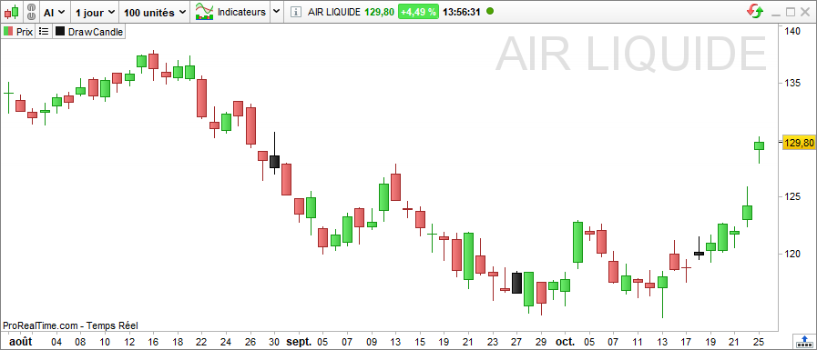
- DRAWCANDLE: Draws a custom candlestick on the chart. Open, high, low and close can be constants or variables.
Example: DRAWCANDLE(Open, High, Low, Close) COLOURED (“black“)
For all the drawing instructions below, the x-axis is expressed as a bar number (Barindex) by default, and the y-axis corresponds to the vertical scale of the values in your graph. You can, however, change this behavior by using the ANCHOR keyword described below.
- DRAWARROW: Draws an arrow pointing to the right. You must define a point for the arrow (x and y axes). You can also choose a color.
Example: DRAWARROW(x1, y1) COLOURED (R, V, B, a)
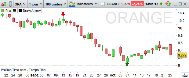
- DRAWARROWUP: Draws an upward-pointing arrow. You must define a point for the arrow (x and y axes). You can also choose a color.
Example: DRAWARROWUP(x1, y1) COLOURED (R, V, B, a)
This is useful for adding visual buying signals.
- DRAWARROWDOWN: Draws an arrow pointing downwards. You must define a point for the arrow (x and y axes). You can also choose a color.
Example: DRAWARROWDOWN(x1, y1) COLOURED (R, V, B, a)
This is useful for adding visual sales signals.
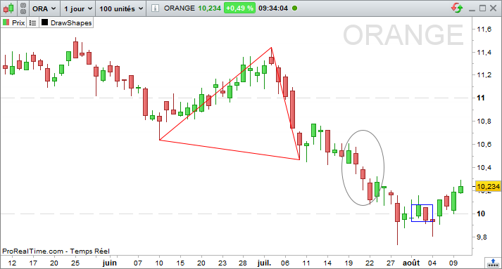
- DRAWRECTANGLE: Draws a rectangle on the graph.
Example: DRAWRECTANGLE(x1, y1, x2, y2) COLOURED (R, V, B, a)
- DRAWTRIANGLE: Draws a triangle on the graph.
Example: DRAWTRIANGLE(x1, y1, x2, y2, x3, y3) COLOURED (R, V, B, a)
- DRAWELLIPSE: Draws an ellipse on the graph.
Example: DRAWELLIPSE(x1, y1, x2, y2) COLOURED (R, V, B, a)
- DRAWPOINT: Draws a point on the graph.
Example: DRAWPOINT (x1, y1, pointSize) COLOURED (R, V, B, a)
- DRAWLINE: Draws a line on the graph.
Example: DRAWLINE (x1, y1, x2, y2) COLOURED (R, V, B, a)
- DRAWHLINE: Draws a horizontal line on the graph.
Example: DRAWHLINE (y1) COLOURED (R, V, B, a)
- DRAWVLINE: Draws a vertical line on the graph.
Example: DRAWVLINE (x1) COLOURED (R, V, B, a)
- DRAWSEGMENT: Draws a segment on the graph.
Example: DRAWSEGMENT (x1, y1, x2, y2) COLOURED (R, V, B, a)
Example: DRAWSEGMENT (Barindex, Close, Barindex[5], Close[5])
- DRAWRAY: Draw half a straight line on the graph
Example: DRAWRAY(x1, y1, x2, y2)
- DRAWTEXT: Adds a text field to the graphic with text of your choice in a specified location. This text can be configured using various style parameters.
Example: DRAWTEXT(“your text”, x1, y1, SERIF, BOLD, 10) COLOURED (R, V, B, a)
Example: DRAWTEXT(value, x1, y1, font, fontStyle, fontSize) COLOURED (R,V,B,a)
Example: DRAWTEXT(value, x1, y1) COLOURED (“green“)
- Here are the different possible values for the font and font style parameters, the font size is between 1 and 30 :
|
Police |
Font style |
DIALOG
|
STANDARD
|
MONOSPACED
|
BOLD
|
SANSERIF
|
BOLDITALIC
|
SERIF
|
ITALIC
|
- DRAWONLASTBARONLY: This parameter allows you to draw objects during the last bar only. This parameter can be used in conjunction with “CALCULATEONLASTBARS” to optimize calculations.
Example: DEFPARAM DRAWONLASTBARONLY = true
Additional parameters
For some of these drawing commands, various additional instructions can be applied in no particular order:
BORDERCOLOR
This instruction defines the color of the border of a drawn object (excluding lines and arrows).
Example 1: DRAWRECTANGLE(Barindex, Close, Barindex[5], Close[5]) BORDERCOLOR(r,g,b,a)
Example 2: DRAWRECTANGLE(Barindex, Close, Barindex[5], Close[5]) BORDERCOLOR(“red”)
ANCHOR
This instruction defines the object’s anchor point when you wish to draw it from a reference other than candlesticks.
DRAWTEXT(Close,n,p)ANCHOR(referencePoint, horizontalShift, verticalShift)
It can take several parameter values:
- Parameter 1: anchor position
| Value | Description |
| TOPLEFT | Fixed at the top left of the chart |
| TOP | Fixed at top of chart (middle) |
| TOPRIGHT | Fixed to the top right of the chart |
| RIGHT | Fixed to the right of the graph (middle) |
| BOTTOMRIGHT | Fixed at bottom right of chart |
| BOTTOM | Fixed at bottom of chart (middle) |
| BOTTOMLEFT | Fixed at bottom left of chart |
| LEFT | Fixed to the left of the graph (middle) |
| MIDDLE | Fixed to the center of the chart |
- Parameter 2: type of value for setting positioning on the horizontal axis
- INDEX: The values entered in the object’s drawing for the horizontal axis will refer to the candlestick barindex.
- XSHIFT: values entered in the object drawing for the horizontal axis will refer to a pixel offset value (positive or negative in relation to an orthonormal frame of reference).
- Parameter 3: type of value to set positioning on the vertical axis
- VALUE: Values entered in the object drawing for the vertical axis will refer to a price.
- YSHIFT: Values entered in the object drawing for the vertical axis will refer to a pixel offset value (positive or negative in relation to an orthonormal frame of reference).
Examples:
- DRAWTEXT(previousClose, -20, -50) ANCHOR(TOPRIGHT, XSHIFT, YSHIFT)
Displays the value of the previousClose variable at the top right of the graph with an offset of -20 on the horizontal axis and -50 on the vertical axis.
- DRAWTEXT(“Top“, Barindex-10, -20) ANCHOR(TOP, INDEX, YSHIFT)
Draws the text “Top” at the top of the chart, offset by -20 on the vertical axis and positioned in the continuity of the 10th barindex before the last.
STYLE
This instruction is used to define a style for objects (excluding arrows) or for returned values.
DRAWRECTANGLE(x1, y1, x2, y2) STYLE(style,lineWidth)
There are different styles:
- DOTTEDLINE: this style transforms the line into a dotted line, there are 5 different configurations representing 5 different dotted line lengths: DOTTEDLINE, DOTTEDLINE1, DOTTEDLINE2, DOTTEDLINE3, DOTTEDLINE4
- LINE: this style restores the default line style (full line).
- HISTOGRAM:this style, only applicable in the RETURN instruction of an indicator, displays the returned values in the form of a histogram.
- POINT:this style, only applicable in the RETURN instruction of an indicator, displays returned values as a point.
- lineWidth, which defines the thickness of the line, will take a value between 1 (thinnest) and 5 (thickest).
Note: for drawing functions, you can specify a date rather than a candlestick index using the DateToBarIndex function, which transforms a date into the nearest associated barindex.
The instruction is written as follows:
DateToBarIndex(Date)
Expected date formats :
- AAAA/ Example: 2022
- AAAAMM / Example: 202208
- YYYYMMDD / Example: 20220815
- AAAAMMJJHH / Example: 2022081517
- AAAAMMJJHHMM / Example: 202208151730
- AAAAMMJJHHMMSS / Example: 20220815173020
Multi-period instructions
ProBuilder lets you work over different time periods in your Backtests, Indicators and ProScreeners, giving you access to more comprehensive data when designing your code.
The instruction is structured as follows:
TIMEFRAME(X TimeUnit , Mode)
With parameters :
- TimeUnit: The type of period selected (see List of available periods)
- X: The value associated with the selected period
- Mode: The selected calculation mode (optional)
Example: TIMEFRAME(1 Hour)
You can use multi-timeframe instructions only to call time units greater than your basic time unit (graph time unit).
Secondary time units must also be a multiple of the base time unit.
So on a 10-minute chart:
You can call a unit of time 20minutes, 1hour, 1day.
You can’t call a unit of time 5 minutes, 17 minutes.
To enter a higher unit of time, use the instruction:
TIMEFRAME(X TimeUnit)
To return to the graph’s basic unit of time, use the following command:
TIMEFRAME(DEFAULT)
You can also indicate the time unit of the basic graph.
The platform editor colors the background of code blocks in higher TimeFrames to help you visualize the pieces of code calculated in each different time unit.
It is also possible to use two calculation modes in a larger unit of time for greater flexibility in your calculations:
TIMEFRAME(X TimeUnit , DEFAULT)
TIMEFRAME(X TimeUnit , UPDATEONCLOSE)
DEFAULT: this is the TimeFrame’s default mode (used when the second parameter is not specified). Calculations in higher time units are performed each time a new price is received in the graph’s base time unit.
UPDATEONCLOSE: calculations contained in a time unit in this mode are performed when the candlestick of the higher time unit closes.
Here’s an example of code showing the difference between the two calculation modes:
// calculation of an average price between opening and closing in the two available modes.
TIMEFRAME(1 Hour)
MidPriceDefault=(Open+ Close)/2
TIMEFRAME(1 Hour, UPDATEONCLOSE)
MidPriceUpdateOnClose=(Open+ Close)/2
Return MidPriceDefault as “Prix Moyen mode Default” COLOURED (“DarkSeaGreen”) ,MidPriceUpdateOnClose as “Prix Moyen mode UpdateOnClose” COLOURED (“DarkRed”)
FCEXXXX 5 minute on October 17, 2022 between 10:00 a.m. and 4:00 p.m.
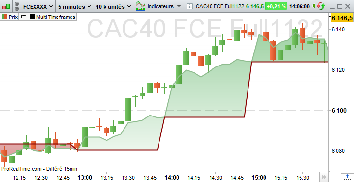
Here we can see that my MidPriceDefault (in green) is updated every 5-minute candlestick, while the MidPriceUpdateOnClose (in red) is updated every 1-hour candlestick.
Note on the use of the TIMEFRAME instruction:
- A variable calculated in one time unit cannot be overwritten by a calculation in another time unit, but variables can be used in all time units contained in the same code.
- There is a limit of 10 TIMEFRAME intraday instructions for automatic trading and backtesting.
- For the ProScreener, only the DEFAULT mode is available, so there’s no need to specify it.
In addition, to guarantee calculation performance on a wide range of real-time values, only a predefined list of available time units is allowed for this module.
For further information, please read the ProScreener documentation.
List of available periods
| Periods | Example |
| Tick / Ticks | TIMEFRAME(1 Tick) |
| sec / Second / Seconds | TIMEFRAME(10 Seconds) |
| mn / Minute / Minutes | TIMEFRAME(5 Minutes) |
| Hour / Hours | TIMEFRAME(1 Hour) |
| Day / Days | TIMEFRAME(5 Days) |
| Week / Weeks | TIMEFRAME(1 Weeks) |
| Month / Months | TIMEFRAME(2 Month) |
| Year / Years | TIMEFRAME(1 Year) |
Data tables
In order to be able to store several values on the same candlestick, or indeed to store values only when necessary, we suggest you use data arrays rather than variables.
A code can contain as many arrays as required, up to a maximum of one million values.
An array is always prefixed with the $ symbol.
| Variable syntax | Array syntax |
| A | $A |
An array starts from index 0 to index 999 999
| Index | 0 | 1 | 2 | 3 | 4 | 5 | 6 | … | 999 999 |
| Value |
To insert a value into an array, simply use
$Tableau[Index] = value
For example, if we want to insert the value of the moving average calculation for period 20 at index 0 of table A, we would write :
$A[0]= Average[20](Close)
To read the value of an array index, use the same principle:
$Table[Index]
For example, if you want to create a condition which checks that the close is greater than the value of the first index of the A array:
Condition= Close >$ A[0]
When a value is inserted at index n of an array, ProBuilder initializes the values to zero for all undefined indices from 0 to n-1, to facilitate use of the data contained in this array.
Specific functions
Several displayboard-specific functions are available to facilitate handling and use:
- ArrayMax($Array): returns the highest value of the defined array. Zeros automatically filled in by ProBuilder are ignored.
- ArrayMin($Array): returns the smallest array value defined. Zeros automatically filled in by ProBuilder are ignored.
- ArraySort($Array,MODE): Sorts the array in ascending order (mode=ASCEND) or descending order (mode=DESCEND). Zeros automatically filled in by ProBuilder will then be removed.
- IsSet($Array[index]): returns 1 if the array index has been set, 0 if it has not. Zeros filled automatically by ProBuilder are not considered to have been defined, so the function will return 0 on these indices.
- LastSet($Array): returns the highest defined index of the array; if no index has been defined in the array, the function will return -1.
- UnSet($Array): Resets the array to 0 by completely deleting its contents.
Please note that, unlike variables and other calculations performed in our language, data arrays are not historized, so it is not possible to retrieve the value of a cell in an array calculated on a previous candlestick.
If you’d like to find out more, we recommend this link from our partner ProRealCode, which explains the use of arrays through various examples.
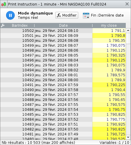
PRINT is a feature that allows you to display in text form the values of any variables or indicators calculated in your code.
This will make it easier for you to understand the calculations performed by your code at runtime.
The results are displayed in tabular form in a new window of your ProRealTime software.
Syntax:
PRINT(Close / 10) AS “my close” FILLCOLOR(255, Barindex / 10, varB, 200) COLOURED(“MidnightBlue”)
Option :
FILLCOLOR: Used to define the background of the Print window box.
COLOURED:Set the color of the value.
AS: Allows you to name the variable displayed in the window.
Colors can be defined using RGB parameters as well as the W3C convention color names. We refer you to the COLOURED section of the ProBuilder keywords, which follows the same rules.
It is of course possible to condition the values to be written when a condition is met.
For example:
MyAverage= Average[10](Close)
IF Close> MyAverage THEN
PRINT (Close-MyAverage) AS “Positive Value
ENDIF
It is possible to display up to 10 different values calculated during the execution of the same code (beyond the first ten values, subsequent values will be ignored).
The displayed values window can contain a history of 200 of the most recent calculations, which are updated as your code performs calculations in real time.
Chapter III: Practical applications
Creating a binary or ternary indicator: why and how?
A binary or ternary indicator is by definition an indicator that can only return two or three possible results (usually 0, 1 or -1). Its main use in a stock market context is to make the verification of the condition that constitutes the indicator immediately identifiable.
Usefulness of a binary or ternary indicator :
- Detect the main Japanese candlestick patterns
- Make it easier to read the graph when trying to identify several conditions
- Putting classic 1-condition alerts on an indicator that incorporates several
- means you’ll have more alerts at your disposal!
- Detecting complex conditions even on the basis of history
- Backtesting made easy
Binary and ternary indicators are constructed using the IF function. We advise you to reread the relative section before continuing.
Let’s illustrate the creation of these indicators to detect price patterns:
Binary indicator: hammer detection
// Hammer detection
Hammer= Close> Open AND High= Close AND (Open-Low)>= 3 *(Close-Open)
IF Hammer THEN
Result= 1
ELSE
Result= 0
ENDIF
RETURN Result AS “Hammer
This simplified code will also give the same results:
Hammer= Close> Open AND High= Close AND (Open-Low)>= 3 *(Close-Open)
RETURN Hammer AS “Hammer
Ternary indicator: detection of golden and deadly crosses
a= ExponentialAverage[10](Close)
b= ExponentialAverage[20](Close)
c= 0
// Golden cross detection
IF a CROSSES OVER b THEN
c= 1
ENDIF
// Deadly cross detection
IF a CROSSES UNDER b THEN
c= -1
ENDIF
RETURN c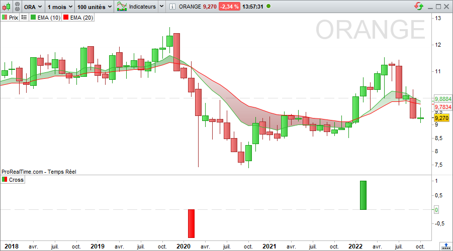
Note: we have displayed the 10- and 20-period exponential moving averages applied to the closing price to highlight the correspondence of the indicator’s results. Further indicators for detecting price patterns can be found in the “Practical Applications” section later in this manual.
Create STOP indicators: track your positions in real time
Indicators can be created to represent STOPS, i.e. potential output levels, defined according to customized parameters.
With the ProBackTest strategy creation module, which is the subject of a separate programming manual, you can define the output levels of a strategy. However, programming an indicator that follows the price of a security is interesting because :
- It displays the stop as a line that updates in real time on the price graph.
- No need to define buy and sell orders (necessary for ProBackTest)
- Real-time alerts can be associated, so that you are immediately alerted to the condition.
Programming Stops will enable you to apply the main commands seen in previous chapters.
In the ProBackTest manual, you’ll also find a number of stop examples for use in investment strategies.
There are 4 categories of stops, which we will review below:
- STOP static profit-taking
- STOP loss static
- Inactivity STOP
- STOP suiveur (trailing stop)
The codes suggested in the following examples represent guidelines for the construction of stop indicators. You’ll need to personalize them using the instructions learned in the previous chapters.
STOP static profit-taking
A Take-Profit STOP is an upper limit on the exit of a position. By definition, this limit is fixed. The user of this STOP then takes profits.
The coded indicator below shows two levels with a position taken on the “Start” date.
- if you’re a buyer, you’ll take into account the top curve representing a 10% gain, or 110% of the price at the time of purchase.
- if you’re a short seller, you’ll take into account the bottom curve, which also represents a 10% gain, i.e. 90% of the price at the time of sale.
In code, this gives :
Below is an example of a STOP to personalize:
// Parameter: StartingTime = 100000
// Correctly set this variable to the time of your position entry
// Price= Price at the time the position is taken (we’ve taken the example of a position entry date set at 10 a.m.)
// If you’re long, you’ll be looking at the top curve. If you’re short, you’ll look at the bottom curve.
// AmplitudeUp represents the Price variation rate used to plot the Take Profit in long positions (default 1.1)
// AmplitudeDown represents the Price variation rate used to plot the Take Profit in the short position (default: 0.9)
IF Time= StartingTime THEN
StopLONG= AmplitudeUp * Price
StopSHORT= AmplitudeDown * Price
ENDIF
RETURN StopLONG COLOURED(0, 0, 0) AS “TakeProfit LONG”, StopSHORT COLOURED(0, 255, 0) AS “TakeProfit SHORT”
STOP loss static
A STOP Loss is the opposite of a STOP Take-Profit: instead of setting an upper exit limit, it sets a lower limit. This STOP is useful for limiting losses to a minimum threshold.
Like Take-Profit, this STOP defines a fixed limit.
The coded indicator below shows two levels with a position taken on the “Start” date.
- if you’re a buyer, you’ll take into account the bottom curve representing a 10% loss, i.e. 90% of the price at the time of purchase.
- if you’re a short seller, you’ll take into account the top curve, which also represents a 10% loss, i.e. 110% of the price at the time of sale.
In code, this gives :
// We define :
// StartingTime = 100000 (we’ve taken the example of a position entry date set to 10 hours)
// Correctly set this variable to the time of your position entry
// Price= position opening price
// AmplitudeUp represents the Price variation rate used to plot the long Stop Loss (default: 0.9)
// AmplitudeDown represents the Price variation rate used to plot the Stop Loss in short positions (default: 1.1)
IF Time= StartingTime THEN
StopLONG= AmplitudeUp * Price
StopSHORT= AmplitudeDown * Price
ENDIF
RETURN StopLONG COLOURED(0, 0, 0) AS “StopLoss LONG”, StopSHORT COLOURED(0, 255, 0) AS “StopLoss SHORT”
STOP inactivity
An inactivity STOP closes the position when earnings have not reached a target (defined in % or points) over a defined period (expressed in number of bars).
Example of an inactivity STOP on an Intraday chart:
This stop is to be used with two indicators:
- the first is juxtaposed on the price curve
- the second to be viewed separately
Indicator1
// MyVolatility = 0.01 corresponds to the relative deviation of the high and low bands of the defined range
IF IntradayBarIndex= 0 THEN
ShortTarget= (1 – MyVolatility) * Close
LongTarget= (1+ MyVolatility) * Close
ENDIF
RETURN ShortTarget AS “ShortTarget”, LongTarget AS “LongTarget”
Indicator2
// We define :
// Position taken at market price
// MyVolatility = 0.01 corresponds to the relative deviation of the high and low bands of the defined range
// NumberOfBars = 20 corresponds to the maximum number of bars over which prices can move before positions are cut (result set to 1).
Result= 0
Cpt= 0
IF IntradayBarIndex= 0 THEN
ShortTarget= (1 – MyVolatility) * Close
LongTarget= (1+ MyVolatility) * Close
ENDIF
FOR i= IntradayBarIndex DOWNTO 1 DO
IF Close[i]>= ShortTarget AND Close[i]<= LongTarget THEN
Cpt= Cpt+ 1
ELSE
Cpt= 0
ENDIF
IF Cpt= NumberOfBars THEN
Result= 1
ENDIF
NEXT
RETURN Result
Trailing stop
A trailing STOP dynamically follows price trends and indicates when the position should be cut.
Below, we suggest two forms of tracking STOP, one corresponding to the Dynamic Stop Loss, the other to the Dynamic Take Profit.
Trailing STOP LOSS (for intraday trading)
// We define :
// StartingTime = 090000 (we’ve taken the example of a position entry date set to 9 o’clock; set this variable correctly to the time of your position entry)
// Position taken at market price
// Amplitude represents the rate of variation of the “Cut” curves with the “Lowest” curves (for example, Amplitude = 0.95).
IF Time= StartingTime THEN
IF lowest[5](Close)< 1.2 * Low THEN
IF lowest[5](Close)>= Close THEN
Cut= Amplitude * lowest[5](Close)
ELSE
Cut= Amplitude * lowest[20](Close)
ENDIF
ELSE
Cut= Amplitude * lowest[20](Close)
ENDIF
ENDIF
RETURN Cut AS “Trailing Stop Loss
Trailing STOP Profit (for intraday trading)
// We define :
// StartingTime = 090000 (we’ve taken the example of a position entry date set to 9 o’clock; set this variable correctly to the time of your position entry)
// The position is taken at the market price
// Amplitude represents the rate of variation of the “Cut” curves with the “Lowest” curves (for example, Amplitude = 1.015).
IF Time= StartingTime THEN
StartingPrice= Close
ENDIF
Price= StartingPrice – AverageTrueRange[10]
TrailingStop= Amplitude * highest[15](Price)
RETURN TrailingStop COLOURED (255, 0, 0) AS “Trailing take profit”
Chapter IV: Exercises
Candlestick figures
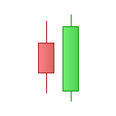
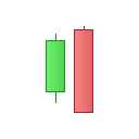
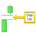
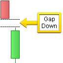
- GAP UP or DOWN
 |
 |
The color of the candlesticks doesn’t matter
We define the amplitude equal to 0.001 as a parameter variable.
A gap is defined by two conditions:
- (today’s opening is strictly higher than the previous day’s closing) or (today’s opening is strictly lower than the previous day’s closing)
- the absolute value of ((today’s opening – previous day’s closing) / previous day’s closing) is strictly greater than the amplitude
// Initialize Amplitude (gap)
Amplitude= 0.001
// Detector initialization
Detector= 0
// Gap Up
// 1st condition for the existence of a gap
IF Low> High[1] THEN
// 2nd gap condition
IF ABS((Low – High[1]) / High[1]) > Amplitude THEN
// Detector behavior
Detector= 1
ENDIF
ENDIF
// Gap Down
// 1st condition for the existence of a gap
IF High< Low[1] THEN
// 2nd gap condition
IF ABS((High – Low[1]) / Low[1]) > Amplitude THEN
// Detector behavior
Detector= -1
ENDIF
ENDIF
// Display result
RETURN Detector AS “Gap detection- Doji (soft version)
 |
A doji is defined by a range strictly greater than 5 times the absolute value of (Open – Close). |
Doji= Range> ABS(Open – Close) * 5
RETURN Doji AS “Doji- Doji (strict version)
 |
The doji is defined by a close equal to the Open. |
Doji= (Open= Close)
RETURN Doji AS “Doji
Indicators
- BODY MOMENTUM
Body Momentum is defined mathematically by :
BodyMomentum = 100 * BodyUp / (BodyUp + BodyDown)
BodyUp (resp. BodyDown) is a counter of the number of bars closing higher (resp. lower) than its opening, over a defined period (let’s take period = 14).
Periods= 14
b= Close – Open
IF BarIndex> Periods THEN
Bup= 0
Bdn= 0
FOR i= 1 TO Periods
IF b[i]> 0 THEN
Bup= Bup+ 1
ELSIF b[i]< 0 THEN
Bdn= Bdn+ 1
ENDIF
NEXT
BM= (Bup / (Bup+ Bdn)) * 100
ELSE
BM= Undefined
ENDIF
RETURN BM AS “Body Momentum- ELLIOT WAVE OSCILLATOR
The Elliot oscillator represents the difference between two moving averages.
The short moving average represents price action, while the long moving average represents the underlying trend.
When prices form a wave 3, prices rise sharply, producing a large value on the oscillator.
In wave 5, prices climb more slowly and the oscillator gives a much lower value.
RETURN Average[5](MedianPrice) – Average[35](MedianPrice) AS “Elliot Wave Oscillator- Williams %R
Here’s an oscillator whose operation is similar to the stochastic oscillator. To plot it, first define 2 curves:
1) 14-period peak-to-peak curve
2) 14-period low-low curve
The %R is then defined as (Close – LowestL ) / (HighestH – LowestL ) * 100
HighestH= highest[14](High)
LowestL= lowest[14](Low)
MyWilliams= (Close – LowestL) / (HighestH – LowestL) * 100
RETURN MyWilliams AS “Williams %R”- Bollinger Bands
We define these bands by framing the 20-bar arithmetic moving average applied to the closing price.
The moving average is bounded above (resp. below) by + (resp. -) 2 times the standard deviation taken from the previous 20 bars of the closing price.
a= Average[20](Close)
// We define the standard deviation
StdDeviation= STD[20](Close)
Bsup= a+ 2 * StdDeviation
Binf= a – 2 * StdDeviation
RETURN a AS “Average”, Bsup AS “Bollinger Up”, Binf AS “Bollinger Down”
You can consult our ProRealTime community on the ProRealCode forum, where you’ll find online documentation and numerous examples.
- Introducing ProBuilder
- Chapter I: Fundamental concepts
- Using ProBuilder
- Programming features of the ProBuilder language
- ProBuilder financial constants
- Price and volume constants adapted to the time unit of the graph
- Daily price constants
- Time constants
- Price-derived constants
- The indefinite constant
- Use of pre-existing indicators
- Adding configurable variables
- Chapter II: ProBuilder functions and instructions
- Control structures
- Conditional instruction IF
- One condition, one result (IF THEN ENDIF)
- One condition, two results (IF THEN ELSE ENDIF)
- Nested conditions
- Multiple conditions (IF THEN ELSIF ELSE ENDIF)
- Iterative loop FOR
- WHILE conditional loop
- BREAK
- CONTINUE
- ONCE
- Mathematical functions
- Common unary and binary functions
- Common mathematical operators
- Graphical comparison functions
- Summation functions
- Statistics functions
- Logic operators
- Keywords ProBuilder
- Drawing commands
- Multi-period instructions
- Data tables
- Chapter III: Practical applications
- Creating a binary or ternary indicator: why and how?
- Create STOP indicators: track your positions in real time
- Chapter IV: Exercises