1. Introduction

The “Center of Gravity of the MACD” is an advanced indicator that combines the popular MACD (Moving Average Convergence Divergence) with the concept of Center of Gravity, providing a more accurate tool for identifying trends and potential turning points. The MACD is one of the most widely used indicators in technical analysis, as it helps to evaluate the direction and strength of a trend, as well as the divergences between price and market momentum. The Center of Gravity of the MACD takes this tool a step further by applying an advanced smoothing method and adding standard deviation bands, which helps identify key overbought and oversold areas.

2. How the Indicator Works

The indicator is built using the classic components of the MACD along with a polynomial adjustment that calculates the center of gravity and bands based on standard deviation and Fibonacci levels. Here’s a breakdown of its main elements:

• MACD and Signal Line: These are calculated in the traditional way, using two exponential moving averages of different periods. The difference between the fast moving average (default 12 periods) and the slow moving average (26 periods) forms the MACD, while a third moving average (default 9 periods) is used to smooth the Signal Line. This difference between the MACD and its Signal Line is used as the core of the indicator to identify trends.
• Center of Gravity (COG): The Center of Gravity is the result of applying a polynomial adjustment to the MACD values, generating a median line that acts as a balance point. This provides a smoother view of the MACD’s movement over time and helps identify more clearly the inflection points where market trends may change.
• Standard Deviation Bands: These are added to the COG to create a channel that delimits the areas where the MACD deviates significantly from its center of gravity. These bands are calculated using the standard deviation of the differences between the MACD and the COG and are multiplied by an adjustable factor (kstd) to determine their width.
• Fibonacci Bands: The Fibonacci bands are added as another layer of information and are based on the multiplication of the standard deviation by a Fibonacci factor (fibband). These additional bands act as potential dynamic support and resistance levels.

3. Interpreting the Indicator

The “Center of Gravity of the MACD” provides detailed information about trend direction and strength, as well as potential reversal points:

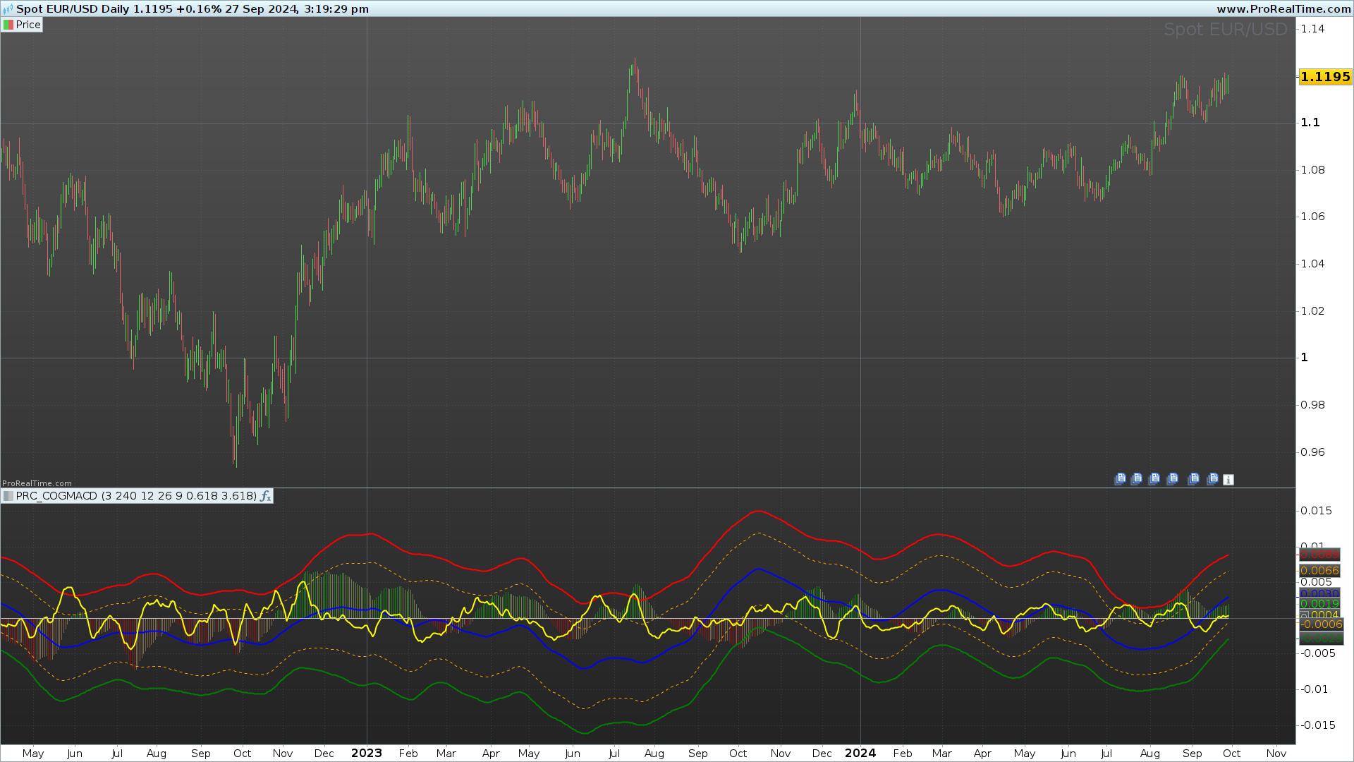
• MACD and COG: When the MACD is above the COG, it indicates an uptrend; when it is below, it suggests a downtrend. Crosses between the MACD and the COG can serve as early signals of a possible trend change.
• MACD Histogram: The histogram, which reflects the difference between the MACD and its Signal Line, changes color to indicate the direction and momentum of the trend:
  • Dark Green: Indicates a strengthening bullish momentum.
  • Light Green: Suggests a weakening bullish momentum.
  • Dark Red: Shows a strengthening bearish momentum.
  • Light Red: Indicates a weakening bearish momentum.
• Standard Deviation and Fibonacci Bands: The bands act as overbought and oversold zones. When the MACD approaches or crosses the upper band, the market might be overbought, and when it nears or crosses the lower band, it could be oversold. The Fibonacci bands provide additional levels that help identify possible reversal areas.

The “Center of Gravity of the MACD” is, therefore, a comprehensive tool that offers a clear view of trends and potential turning points in the market.

4. Configuring the Indicator in ProRealTime

The “Center of Gravity of the MACD” is a flexible and customizable indicator that can adapt to different trading styles thanks to its configurable parameters. Below are the main parameters that can be adjusted in ProRealTime:

• fma (Fast Moving Average): Number of periods for the fast moving average used to calculate the MACD. The default value is 12.
• sma (Slow Moving Average): Number of periods for the slow moving average used to calculate the MACD. The default value is 26.
• sigma: Number of periods for the moving average that smooths the MACD Signal Line. The default value is 9.
• m: Controls the degree of the polynomial used to calculate the Center of Gravity. A higher value makes the adjustment more sensitive to variations in the MACD.
• p: Defines the number of historical bars used to calculate the Center of Gravity. A higher value generates a smoother center, less sensitive to recent fluctuations.
• kstd: Multiplication factor applied to the standard deviation to calculate the upper and lower bands. A higher value will generate wider bands, reducing overbought or oversold signals.
• fibband: Fibonacci-based factor used to calculate the additional bands. The default value is 0.618, representing the golden ratio.

These parameters can be adjusted according to the nature of the asset you are analyzing and your investment horizon. For example, in a more volatile market, you might want to increase the “kstd” value to get more precise signals.

5. Advantages and Limitations

Advantages:

• Combination of Multiple Tools: The Center of Gravity of the MACD combines MACD analysis with smoothing concepts and standard deviation bands, making it a very complete indicator.
• Identification of Trends and Extreme Zones: The bands provide an effective way to identify potential overbought and oversold zones, while the COG helps identify trend direction.
• Flexibility: The adjustable parameters allow the indicator to adapt to different financial instruments and trading styles, from intraday trading to swing trading.

Limitations:

• Complexity: The amount of information provided can be overwhelming for beginner traders, especially if they are not familiar with using the MACD and standard deviation concepts.
• Parameter Dependence: As with many technical indicators, the results can vary significantly depending on the parameter values. This means users need to carefully adjust these values to obtain accurate signals.
• Signal Lag: Like other moving average-based indicators, the COG and standard deviation bands can show a certain lag relative to price action.

6. Conclusion

The “Center of Gravity of the MACD” is a powerful and versatile indicator that combines the effectiveness of the MACD with a more advanced approach to smoothing and standard deviation bands. By adding the concept of center of gravity and Fibonacci bands, it provides traders with a clearer and more detailed view of market trends and momentum, as well as potential reversal areas.

This indicator is especially useful for traders looking for a comprehensive tool that not only helps them identify the trend direction but also offers precise entry and exit points based on overbought and oversold zones. However, as with any technical indicator, it is essential to understand its limitations and adjust the parameters according to market characteristics and the instrument being analyzed.

In summary, the Center of Gravity of the MACD is an excellent addition to any trading strategy, and its flexibility and customization make it a valuable tool for both beginner and experienced traders.

//----------------------------------------------------------------//
// PRC COGMACD
//version = 0
//23.07.2024
//Iván González @ www.prorealcode.com
//Sharing ProRealTime knowledge
//----------------------------------------------------------------//
//-----Inputs-----------------------------------------------------//
m = 3
p = 240

fma = 12
sma = 26
sigma = 9

fibband = 0.618
kstd = 3.618
//----------------------------------------------------------------//
//-----MACD calculation-------------------------------------------//
// Calculate the MACD and Signal line
myMacd = macd[fma, sma, sigma](close)
signal = MACDSignal[fma, sma, sigma](close)
MacdMiddle = (myMacd + signal) / 2
//----------------------------------------------------------------//
nn = m + 1

// Calculate the sx array which contains the sum of powers of n
for mi = 1 to nn * 2 - 2 do
sum = 0
for n = 0 to p do
sum = sum + pow(n, mi)
next
$sx[mi + 1] = sum
next
//----------------------------------------------------------------//
// Calculate the b array using MacdMiddle values
for mi = 1 to nn do
sum = 0
for n = 0 to p do
if mi = 1 then
sum = sum + MacdMiddle[n]
else
sum = sum + MacdMiddle[n] * pow(n, mi - 1)
endif
next
$b[mi] = sum
next
//----------------------------------------------------------------//
// Populate the ai matrix using the sx values
for jj = 1 to nn do
for ii = 1 to nn do
kk = ii + jj - 1
$ai[(ii - 1) * nn + jj] = $sx[kk]
next
next
//----------------------------------------------------------------//
// Apply Gauss method to solve the system of equations
for kk = 1 to nn - 1 do
ll = 0
mm = 0
qq = 0
tt = 0
for ii = kk to nn do
if abs($ai[(ii - 1) * nn + kk]) > mm then
mm = abs($ai[(ii - 1) * nn + kk])
ll = ii
endif
next
if ll <> kk then
for jj = 1 to nn do
tt = $ai[(kk - 1) * nn + jj]
$ai[(kk - 1) * nn + jj] = $ai[(ll - 1) * nn + jj]
$ai[(ll - 1) * nn + jj] = tt
next
tt = $b[kk]
$b[kk] = $b[ll]
$b[ll] = tt
endif
for ii = kk + 1 to nn do
qq = $ai[(ii - 1) * nn + kk] / $ai[(kk - 1) * nn + kk]
for jj = 1 to nn do
if jj = kk then
$ai[(ii - 1) * nn + jj] = 0
else
$ai[(ii - 1) * nn + jj] = $ai[(ii - 1) * nn + jj] - qq * $ai[(kk - 1) * nn + jj]
endif
next
$b[ii] = $b[ii] - qq * $b[kk]
next
next
//----------------------------------------------------------------//
// Calculate the coefficients of the polynomial using back substitution
$x[nn] = $b[nn] / $ai[(nn - 1) * nn + nn]

for ii = nn - 1 downto 1 do
tt = 0
for jj = 1 to nn - ii do
tt = tt + $ai[(ii - 1) * nn + (ii + jj)] * $x[ii + jj]
next
$x[ii] = (1 / $ai[(ii - 1) * nn + ii]) * ($b[ii] - tt)
next
//----------------------------------------------------------------//
// Calculate the Center of Gravity (COG) and the standard deviation bands
sq = 0.0

for n = 0 to p do
sum = 0
for kk = 1 to m do
sum = sum + $x[kk + 1] * pow(n, kk)
next

// Center of Gravity calculation
$fx[n] = $x[1] + sum

// Accumulate the squared differences for standard deviation
sq = sq + pow(MacdMiddle[n] - $fx[n], 2)

// Calculate standard deviation
st = sqrt(sq / (p + 1)) * kstd

// Calculate the bands based on standard deviation
$sqh[n] = $fx[n] + st
$sql[n] = $fx[n] - st
$stdh[n] = $fx[n] + (fibband * st)
$stdl[n] = $fx[n] - (fibband * st)
next
//----------------------------------------------------------------//
return $fx[p] as "Center of Gravity" coloured("blue") style(line,2), $sqh[p] as "Upper Band" coloured("red") style(line,2), $sql[p] as "Lower Band" coloured("green") style(line,2), $stdh[p] as "Upper Fibonacci Band" coloured("orange") style(dottedline,1), $stdl[p] as "Lower Fibonacci Band" coloured("orange") style(dottedline,1), myMacd coloured("yellow") style(line,2), 0 as "zero"