Thanks Derek, I came across this article too. I think the following two articles by:
http://www.brainyforex.com/position-sizing-methods.html and http://traders.com/Documentation/FEEDbk_docs/1998/07/Abstracts_new/Zamansky/Zamansky9807.html
might help @Nicolas to code a solution that gets rid of the problem of “wild swings” in equity and large drawdowns that can occur even when using Ralph Vince’s Optimal F.
BRAINY FOREX:
Optimal F
Like the Kelly formula, optimal f position sizing method is a specialized form of fixed fractional (fixed risk) position sizing. Optimal f position sizing method uses the fixed fraction that maximizes the geometric rate of equity growth. This method was developed by Ralph Vince as a more accurate version of the Kelly formula. Unfortunately, optimal f has many of the same drawbacks as the Kelly formula. Namely, the optimal f value often results in drawdowns that are too large for most traders to tolerate. As with the Kelly formula, the position size based on the optimal f is often so high that it’s limited by margin requirements.
The optimal f value is calculated according to an iterative procedure that maximizes the geometric growth rate for the current sequence of trades. The calculation for the position size is the same as for the Kelly formula except that the optimal f value is used in place of the Kelly f value. The trade risk is taken as the largest historical loss per unit. As with the Kelly formula, optimal f position sizing is included primarily for educational purposes.
Secure F
Leo Zamansky and David Stendahl tried to overcome large drawdowns Optimal f by adding a special limit of maximal allowable drawdown. Secure F solves a task:
Net Profit -> Max (similarly Optimal f) under condition Max Drawdown <= Max Allowed Drawdown.
The difference between the Secure F and the Optimal f position sizing methods is that in case of Secure F the drawdown will be taken into account. Value of Secure F can never be higher that the value of Optimal f.
Number of units = (Secure F * Current Capital/starting risk per unity of assets)/Security Price
where starting risk = maximal loss at trade(in %).
Example:
Current Capital = $2,000,000 ($10,000 with margin factor of 200).

Currency Price = 1.2785

Max DrawDown = 20% (value of maximal allowed DrawDown)

Secure F = 0.10 (value of maximal allowed DrawDown)

Maximal Loss at trade = 50%

In this case you can buy (0.1 * 2,000,000/0.5)/1.2785 = 312,867/0.2 = 156,433 units.($200,000)
———————————————————————————————————————————————————————————————–
TRADERS . COM
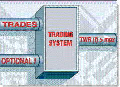
Here’s how to find a new fractional value of capital to invest in every trade to maximize returns subject to a constraint on drawdown, using a variation of the optimal f money management strategy:
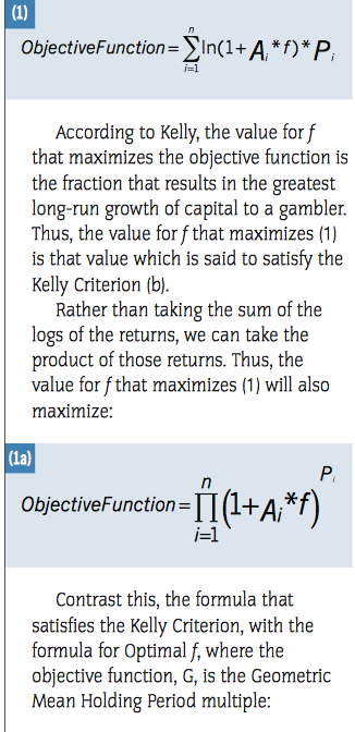
Vince introduces optimal f, and to find the value of optimal f, we need to maximize what Vince calls terminal wealth relative (TWR). The problem can be formulated thus:
TWR(f) -> max
where TWR(f)=(HPR1(f))((HPR2(f))(...(HPRn(f))

HPRi(f)=1+(f((-Return on the trade i)/(Return on the worst losing trade))

HPR = Holding period return
(Please see Zaminsky screenshot)
———————————————————————————————————————————————————————————————–
NOTE:
The IFTA conclusion below also addresses the issue of not knowing where the the optimal point will be in the future (we’re using past probabilities).
A solution has been provided (see italics) in the IFTA Research Paper’s Conclusion: (page 26)
“The above findings (singularities and discontinuities in geometric growth) have important implications for a trader wishing to implement Optimal f in his future trading. One of the major impediments to implementing the usage of Optimal f for geometric growth in trading is the lack of knowledge as to where the optimal point will be in the future.
Since the Optimal f case will necessarily bound the future optimal point between zero and p (the sum of the probabilities of the winning scenarios), the trader need only perceive what p will be in the future. From there, trading a value for f of p/2 will minimize the cost of missing the peak of the Optimal f curve in the future.
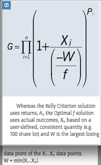
This occurs because each point along the Optimal f curve varies with the increase in the number of plays (time), T, as GT, where G is the geometric mean holding period multiple as given in Equation (2)(see previous screenshot). Thus, at T=2, the price paid for being at any future f value other than the optimal value is squared, at T=3, the penalty is cubed. Just as with the measure of statistical variance, outliers cost proportionally more. Although the trader cannot judge what will be the future value for Optimal f, by using the value of p/2 as the future estimate of the Optimal f, the trader minimizes this cost and is able to make a “best guess” estimate of what the future value for Optimal f will be.
Note that the trader uses a predicted value for p in determining his future “best guess” for f . The greatest amount the trader might miss actually is the optimal point in the future and is the greater of p/2 or what we call p’, which is what p actually comes in as in the future window, p’ – p/2. These extreme cases manifest when the trader opts for f = p/2 and the future Optimal f=0, or, the trader opts for f = p/2 and the future Optimal f=p’. Thus, the greatest outlier, when the trader is opting to use a “best guess” for his future Optimal f = p /2 is minimized as the greater of p/2 and p’-p/2.
Because the Kelly Criterion Solution is unbounded to the right, we are not afforded this outcome unless, we convert it to its Optimal f analog.
At no losses, the Kelly Criterion solution is infinitely high, and only by convention can we conclude that the corresponding Optimal f is 1.0. The point of singularity we witness in Optimal f is mathematical, the discontinuity, by convention.”