Please convert Code To ProRealTime: Code source from trading view indicator

• 03/10/2023 at 6:10 PM #211330
  JackSheldrick

  // This source code is subject to the terms of the Mozilla Public License 2.0 at https://mozilla.org/MPL/2.0/
  // ©jdehorty

  // @version=5
  indicator(‘Machine Learning: Lorentzian Classification’, ‘Lorentzian Classification’, true, precision=4, max_labels_count=500)

  import jdehorty/MLExtensions/2 as ml
  import jdehorty/KernelFunctions/2 as kernels

  // ====================
  // ==== Background ====
  // ====================

  // When using Machine Learning algorithms like K-Nearest Neighbors, choosing an
  // appropriate distance metric is essential. Euclidean Distance is often used as
  // the default distance metric, but it may not always be the best choice. This is
  // because market data is often significantly impacted by proximity to significant
  // world events such as FOMC Meetings and Black Swan events. These major economic
  // events can contribute to a warping effect analogous a massive object’s
  // gravitational warping of Space-Time. In financial markets, this warping effect
  // operates on a continuum, which can analogously be referred to as “Price-Time”.

  // To help to better account for this warping effect, Lorentzian Distance can be
  // used as an alternative distance metric to Euclidean Distance. The geometry of
  // Lorentzian Space can be difficult to visualize at first, and one of the best
  // ways to intuitively understand it is through an example involving 2 feature
  // dimensions (z=2). For purposes of this example, let’s assume these two features
  // are Relative Strength Index (RSI) and the Average Directional Index (ADX). In
  // reality, the optimal number of features is in the range of 3-8, but for the sake
  // of simplicity, we will use only 2 features in this example.

  // Fundamental Assumptions:
  // (1) We can calculate RSI and ADX for a given chart.
  // (2) For simplicity, values for RSI and ADX are assumed to adhere to a Gaussian
  // distribution in the range of 0 to 100.
  // (3) The most recent RSI and ADX value can be considered the origin of a coordinate
  // system with ADX on the x-axis and RSI on the y-axis.

  // Distances in Euclidean Space:
  // Measuring the Euclidean Distances of historical values with the most recent point
  // at the origin will yield a distribution that resembles Figure 1 (below).

  // [RSI]
  // |
  // |
  // |
  // …:::….
  // .:.:::••••••:::•::..
  // .:•:.:•••::::••::••….::.
  // ….:••••:••••••••::••:…:•.
  // …:.::::::•••:::•••:•••::.:•..
  // ::•:.:•:•••••••:.:•::::::…:..
  // |——–.:•••..•••••••:••:…:::•:•:..:..———-[ADX]
  // 0 :•:….:•••••::.:::•••::••:…..
  // ::….:.:••••••••:•••::••::..:.
  // .:…:••:::••••••••::•••….:
  // ::….:…..:•::•••:::::..
  // ..:..::••..::::..:•:..
  // .::..:::…..:
  // |
  // |
  // |
  // |
  // _|_ 0
  //
  // Figure 1: Neighborhood in Euclidean Space

  // Distances in Lorentzian Space:
  // However, the same set of historical values measured using Lorentzian Distance will
  // yield a different distribution that resembles Figure 2 (below).

  //
  // [RSI]
  // ::.. | ..:::
  // ….. | ……
  // .••••::. | :••••••.
  // .:•••••:. | :::••••••.
  // .•••••:… | .::.••••••.
  // .::•••••::.. | :..••••••..
  // .:•••••••::………::••••••:..
  // ..::::••••.•••••••.•••••••:.
  // …:•••••••.•••••••••::.
  // .:..••.••••••.••••..
  // |—————.:•••••••••••••••••.—————[ADX]
  // 0 .:•:•••.••••••.•••••••.
  // .••••••••••••••••••••••••:.
  // .:••••••••••::..::.::••••••••:.
  // .::••••••::. | .::•••:::.
  // .:••••••.. | :••••••••.
  // .:••••:… | ..•••••••:.
  // ..:••::.. | :.•••••••.
  // .:•…. | …::.:••.
  // …:.. | :…:••.
  // :::. | ..::
  // _|_ 0
  //
  // Figure 2: Neighborhood in Lorentzian Space

  // Observations:
  // (1) In Lorentzian Space, the shortest distance between two points is not
  // necessarily a straight line, but rather, a geodesic curve.
  // (2) The warping effect of Lorentzian distance reduces the overall influence
  // of outliers and noise.
  // (3) Lorentzian Distance becomes increasingly different from Euclidean Distance
  // as the number of nearest neighbors used for comparison increases.

  // ======================
  // ==== Custom Types ====
  // ======================

  // This section uses PineScript’s new Type syntax to define important data structures
  // used throughout the script.

  type Settings
  float source
  int neighborsCount
  int maxBarsBack
  int featureCount
  int colorCompression
  bool showExits
  bool useDynamicExits

  type Label
  int long
  int short
  int neutral

  type FeatureArrays
  array<float> f1
  array<float> f2
  array<float> f3
  array<float> f4
  array<float> f5

  type FeatureSeries
  float f1
  float f2
  float f3
  float f4
  float f5

  type MLModel
  int firstBarIndex
  array<int> trainingLabels
  int loopSize
  float lastDistance
  array<float> distancesArray
  array<int> predictionsArray
  int prediction

  type FilterSettings
  bool useVolatilityFilter
  bool useRegimeFilter
  bool useAdxFilter
  float regimeThreshold
  int adxThreshold

  type Filter
  bool volatility
  bool regime
  bool adx

  // ==========================
  // ==== Helper Functions ====
  // ==========================

  series_from(feature_string, _close, _high, _low, _hlc3, f_paramA, f_paramB) =>
  switch feature_string
  “RSI” => ml.n_rsi(_close, f_paramA, f_paramB)
  “WT” => ml.n_wt(_hlc3, f_paramA, f_paramB)
  “CCI” => ml.n_cci(_close, f_paramA, f_paramB)
  “ADX” => ml.n_adx(_high, _low, _close, f_paramA)

  get_lorentzian_distance(int i, int featureCount, FeatureSeries featureSeries, FeatureArrays featureArrays) =>
  switch featureCount
  5 => math.log(1+math.abs(featureSeries.f1 – array.get(featureArrays.f1, i))) +
  math.log(1+math.abs(featureSeries.f2 – array.get(featureArrays.f2, i))) +
  math.log(1+math.abs(featureSeries.f3 – array.get(featureArrays.f3, i))) +
  math.log(1+math.abs(featureSeries.f4 – array.get(featureArrays.f4, i))) +
  math.log(1+math.abs(featureSeries.f5 – array.get(featureArrays.f5, i)))
  4 => math.log(1+math.abs(featureSeries.f1 – array.get(featureArrays.f1, i))) +
  math.log(1+math.abs(featureSeries.f2 – array.get(featureArrays.f2, i))) +
  math.log(1+math.abs(featureSeries.f3 – array.get(featureArrays.f3, i))) +
  math.log(1+math.abs(featureSeries.f4 – array.get(featureArrays.f4, i)))
  3 => math.log(1+math.abs(featureSeries.f1 – array.get(featureArrays.f1, i))) +
  math.log(1+math.abs(featureSeries.f2 – array.get(featureArrays.f2, i))) +
  math.log(1+math.abs(featureSeries.f3 – array.get(featureArrays.f3, i)))
  2 => math.log(1+math.abs(featureSeries.f1 – array.get(featureArrays.f1, i))) +
  math.log(1+math.abs(featureSeries.f2 – array.get(featureArrays.f2, i)))

  // ================
  // ==== Inputs ====
  // ================

  // Settings Object: General User-Defined Inputs
  Settings settings =
  Settings.new(
  input.source(title=’Source’, defval=close, group=”General Settings”, tooltip=”Source of the input data”),
  input.int(title=’Neighbors Count’, defval=8, group=”General Settings”, minval=1, maxval=100, step=1, tooltip=”Number of neighbors to consider”),
  input.int(title=”Max Bars Back”, defval=2000, group=”General Settings”),
  input.int(title=”Feature Count”, defval=5, group=”Feature Engineering”, minval=2, maxval=5, tooltip=”Number of features to use for ML predictions.”),
  input.int(title=”Color Compression”, defval=1, group=”General Settings”, minval=1, maxval=10, tooltip=”Compression factor for adjusting the intensity of the color scale.”),
  input.bool(title=”Show Default Exits”, defval=false, group=”General Settings”, tooltip=”Default exits occur exactly 4 bars after an entry signal. This corresponds to the predefined length of a trade during the model’s training process.”, inline=”exits”),
  input.bool(title=”Use Dynamic Exits”, defval=false, group=”General Settings”, tooltip=”Dynamic exits attempt to let profits ride by dynamically adjusting the exit threshold based on kernel regression logic.”, inline=”exits”)
  )

  // Trade Stats Settings
  // Note: The trade stats section is NOT intended to be used as a replacement for proper backtesting. It is intended to be used for calibration purposes only.
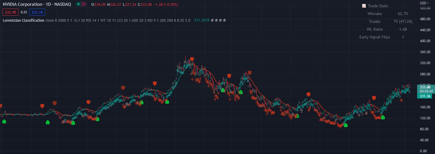
  showTradeStats = input.bool(true, ‘Show Trade Stats’, tooltip=’Displays the trade stats for a given configuration. Useful for optimizing the settings in the Feature Engineering section. This should NOT replace backtesting and should be used for calibration purposes only. Early Signal Flips represent instances where the model changes signals before 4 bars elapses; high values can indicate choppy (ranging) market conditions.’, group=”General Settings”)
  useWorstCase = input.bool(false, “Use Worst Case Estimates”, tooltip=”Whether to use the worst case scenario for backtesting. This option can be useful for creating a conservative estimate that is based on close prices only, thus avoiding the effects of intrabar repainting. This option assumes that the user does not enter when the signal first appears and instead waits for the bar to close as confirmation. On larger timeframes, this can mean entering after a large move has already occurred. Leaving this option disabled is generally better for those that use this indicator as a source of confluence and prefer estimates that demonstrate discretionary mid-bar entries. Leaving this option enabled may be more consistent with traditional backtesting results.”, group=”General Settings”)

  // Settings object for user-defined settings
  FilterSettings filterSettings =
  FilterSettings.new(
  input.bool(title=”Use Volatility Filter”, defval=true, tooltip=”Whether to use the volatility filter.”, group=”Filters”),
  input.bool(title=”Use Regime Filter”, defval=true, group=”Filters”, inline=”regime”),
  input.bool(title=”Use ADX Filter”, defval=false, group=”Filters”, inline=”adx”),
  input.float(title=”Threshold”, defval=-0.1, minval=-10, maxval=10, step=0.1, tooltip=”Whether to use the trend detection filter. Threshold for detecting Trending/Ranging markets.”, group=”Filters”, inline=”regime”),
  input.int(title=”Threshold”, defval=20, minval=0, maxval=100, step=1, tooltip=”Whether to use the ADX filter. Threshold for detecting Trending/Ranging markets.”, group=”Filters”, inline=”adx”)
  )

  // Filter object for filtering the ML predictions
  Filter filter =
  Filter.new(
  ml.filter_volatility(1, 10, filterSettings.useVolatilityFilter),
  ml.regime_filter(ohlc4, filterSettings.regimeThreshold, filterSettings.useRegimeFilter),
  ml.filter_adx(settings.source, 14, filterSettings.adxThreshold, filterSettings.useAdxFilter)
  )

  // Feature Variables: User-Defined Inputs for calculating Feature Series.
  f1_string = input.string(title=”Feature 1″, options=[“RSI”, “WT”, “CCI”, “ADX”], defval=”RSI”, inline = “01”, tooltip=”The first feature to use for ML predictions.”, group=”Feature Engineering”)
  f1_paramA = input.int(title=”Parameter A”, tooltip=”The primary parameter of feature 1.”, defval=14, inline = “02”, group=”Feature Engineering”)
  f1_paramB = input.int(title=”Parameter B”, tooltip=”The secondary parameter of feature 2 (if applicable).”, defval=1, inline = “02”, group=”Feature Engineering”)
  f2_string = input.string(title=”Feature 2″, options=[“RSI”, “WT”, “CCI”, “ADX”], defval=”WT”, inline = “03”, tooltip=”The second feature to use for ML predictions.”, group=”Feature Engineering”)
  f2_paramA = input.int(title=”Parameter A”, tooltip=”The primary parameter of feature 2.”, defval=10, inline = “04”, group=”Feature Engineering”)
  f2_paramB = input.int(title=”Parameter B”, tooltip=”The secondary parameter of feature 2 (if applicable).”, defval=11, inline = “04”, group=”Feature Engineering”)
  f3_string = input.string(title=”Feature 3″, options=[“RSI”, “WT”, “CCI”, “ADX”], defval=”CCI”, inline = “05”, tooltip=”The third feature to use for ML predictions.”, group=”Feature Engineering”)
  f3_paramA = input.int(title=”Parameter A”, tooltip=”The primary parameter of feature 3.”, defval=20, inline = “06”, group=”Feature Engineering”)
  f3_paramB = input.int(title=”Parameter B”, tooltip=”The secondary parameter of feature 3 (if applicable).”, defval=1, inline = “06”, group=”Feature Engineering”)
  f4_string = input.string(title=”Feature 4″, options=[“RSI”, “WT”, “CCI”, “ADX”], defval=”ADX”, inline = “07”, tooltip=”The fourth feature to use for ML predictions.”, group=”Feature Engineering”)
  f4_paramA = input.int(title=”Parameter A”, tooltip=”The primary parameter of feature 4.”, defval=20, inline = “08”, group=”Feature Engineering”)
  f4_paramB = input.int(title=”Parameter B”, tooltip=”The secondary parameter of feature 4 (if applicable).”, defval=2, inline = “08”, group=”Feature Engineering”)
  f5_string = input.string(title=”Feature 5″, options=[“RSI”, “WT”, “CCI”, “ADX”], defval=”RSI”, inline = “09”, tooltip=”The fifth feature to use for ML predictions.”, group=”Feature Engineering”)
  f5_paramA = input.int(title=”Parameter A”, tooltip=”The primary parameter of feature 5.”, defval=9, inline = “10”, group=”Feature Engineering”)
  f5_paramB = input.int(title=”Parameter B”, tooltip=”The secondary parameter of feature 5 (if applicable).”, defval=1, inline = “10”, group=”Feature Engineering”)

  // FeatureSeries Object: Calculated Feature Series based on Feature Variables
  featureSeries =
  FeatureSeries.new(
  series_from(f1_string, close, high, low, hlc3, f1_paramA, f1_paramB), // f1
  series_from(f2_string, close, high, low, hlc3, f2_paramA, f2_paramB), // f2
  series_from(f3_string, close, high, low, hlc3, f3_paramA, f3_paramB), // f3
  series_from(f4_string, close, high, low, hlc3, f4_paramA, f4_paramB), // f4
  series_from(f5_string, close, high, low, hlc3, f5_paramA, f5_paramB) // f5
  )

  // FeatureArrays Variables: Storage of Feature Series as Feature Arrays Optimized for ML
  // Note: These arrays cannot be dynamically created within the FeatureArrays Object Initialization and thus must be set-up in advance.
  var f1Array = array.new_float()
  var f2Array = array.new_float()
  var f3Array = array.new_float()
  var f4Array = array.new_float()
  var f5Array = array.new_float()
  array.push(f1Array, featureSeries.f1)
  array.push(f2Array, featureSeries.f2)
  array.push(f3Array, featureSeries.f3)
  array.push(f4Array, featureSeries.f4)
  array.push(f5Array, featureSeries.f5)

  // FeatureArrays Object: Storage of the calculated FeatureArrays into a single object
  featureArrays =
  FeatureArrays.new(
  f1Array, // f1
  f2Array, // f2
  f3Array, // f3
  f4Array, // f4
  f5Array // f5
  )

  // Label Object: Used for classifying historical data as training data for the ML Model
  Label direction =
  Label.new(
  long=1,
  short=-1,
  neutral=0
  )

  // Derived from General Settings
  maxBarsBackIndex = last_bar_index >= settings.maxBarsBack ? last_bar_index – settings.maxBarsBack : 0

  // EMA Settings
  useEmaFilter = input.bool(title=”Use EMA Filter”, defval=false, group=”Filters”, inline=”ema”)
  emaPeriod = input.int(title=”Period”, defval=200, minval=1, step=1, group=”Filters”, inline=”ema”, tooltip=”The period of the EMA used for the EMA Filter.”)
  isEmaUptrend = useEmaFilter ? close > ta.ema(close, emaPeriod) : true
  isEmaDowntrend = useEmaFilter ? close < ta.ema(close, emaPeriod) : true
  useSmaFilter = input.bool(title=”Use SMA Filter”, defval=false, group=”Filters”, inline=”sma”)
  smaPeriod = input.int(title=”Period”, defval=200, minval=1, step=1, group=”Filters”, inline=”sma”, tooltip=”The period of the SMA used for the SMA Filter.”)
  isSmaUptrend = useSmaFilter ? close > ta.sma(close, smaPeriod) : true
  isSmaDowntrend = useSmaFilter ? close < ta.sma(close, smaPeriod) : true

  // Nadaraya-Watson Kernel Regression Settings
  useKernelFilter = input.bool(true, “Trade with Kernel”, group=”Kernel Settings”, inline=”kernel”)
  showKernelEstimate = input.bool(true, “Show Kernel Estimate”, group=”Kernel Settings”, inline=”kernel”)
  useKernelSmoothing = input.bool(false, “Enhance Kernel Smoothing”, tooltip=”Uses a crossover based mechanism to smoothen kernel color changes. This often results in less color transitions overall and may result in more ML entry signals being generated.”, inline=’1′, group=’Kernel Settings’)
  h = input.int(8, ‘Lookback Window’, minval=3, tooltip=’The number of bars used for the estimation. This is a sliding value that represents the most recent historical bars. Recommended range: 3-50′, group=”Kernel Settings”, inline=”kernel”)
  r = input.float(8., ‘Relative Weighting’, step=0.25, tooltip=’Relative weighting of time frames. As this value approaches zero, the longer time frames will exert more influence on the estimation. As this value approaches infinity, the behavior of the Rational Quadratic Kernel will become identical to the Gaussian kernel. Recommended range: 0.25-25′, group=”Kernel Settings”, inline=”kernel”)
  x = input.int(25, “Regression Level”, tooltip=’Bar index on which to start regression. Controls how tightly fit the kernel estimate is to the data. Smaller values are a tighter fit. Larger values are a looser fit. Recommended range: 2-25′, group=”Kernel Settings”, inline=”kernel”)
  lag = input.int(2, “Lag”, tooltip=”Lag for crossover detection. Lower values result in earlier crossovers. Recommended range: 1-2″, inline=’1′, group=’Kernel Settings’)

  // Display Settings
  showBarColors = input.bool(true, “Show Bar Colors”, tooltip=”Whether to show the bar colors.”, group=”Display Settings”)
  showBarPredictions = input.bool(defval = true, title = “Show Bar Prediction Values”, tooltip = “Will show the ML model’s evaluation of each bar as an integer.”, group=”Display Settings”)
  useAtrOffset = input.bool(defval = false, title = “Use ATR Offset”, tooltip = “Will use the ATR offset instead of the bar prediction offset.”, group=”Display Settings”)
  barPredictionsOffset = input.float(0, “Bar Prediction Offset”, minval=0, tooltip=”The offset of the bar predictions as a percentage from the bar high or close.”, group=”Display Settings”)

  // =================================
  // ==== Next Bar Classification ====
  // =================================

  // This model specializes specifically in predicting the direction of price action over the course of the next 4 bars.
  // To avoid complications with the ML model, this value is hardcoded to 4 bars but support for other training lengths may be added in the future.
  src = settings.source
  y_train_series = src[4] < src[0] ? direction.short : src[4] > src[0] ? direction.long : direction.neutral
  var y_train_array = array.new_int(0)

  // Variables used for ML Logic
  var predictions = array.new_float(0)
  var prediction = 0.
  var signal = direction.neutral
  var distances = array.new_float(0)

  array.push(y_train_array, y_train_series)

  // =========================
  // ==== Core ML Logic ====
  // =========================

  // Approximate Nearest Neighbors Search with Lorentzian Distance:
  // A novel variation of the Nearest Neighbors (NN) search algorithm that ensures a chronologically uniform distribution of neighbors.

  // In a traditional KNN-based approach, we would iterate through the entire dataset and calculate the distance between the current bar
  // and every other bar in the dataset and then sort the distances in ascending order. We would then take the first k bars and use their
  // labels to determine the label of the current bar.

  // There are several problems with this traditional KNN approach in the context of real-time calculations involving time series data:
  // – It is computationally expensive to iterate through the entire dataset and calculate the distance between every historical bar and
  // the current bar.
  // – Market time series data is often non-stationary, meaning that the statistical properties of the data change slightly over time.
  // – It is possible that the nearest neighbors are not the most informative ones, and the KNN algorithm may return poor results if the
  // nearest neighbors are not representative of the majority of the data.

  // Previously, the user @capissimo attempted to address some of these issues in several of his PineScript-based KNN implementations by:
  // – Using a modified KNN algorithm based on consecutive furthest neighbors to find a set of approximate “nearest” neighbors.
  // – Using a sliding window approach to only calculate the distance between the current bar and the most recent n bars in the dataset.

  // Of these two approaches, the latter is inherently limited by the fact that it only considers the most recent bars in the overall dataset.

  // The former approach has more potential to leverage historical price action, but is limited by:
  // – The possibility of a sudden “max” value throwing off the estimation
  // – The possibility of selecting a set of approximate neighbors that are not representative of the majority of the data by oversampling
  // values that are not chronologically distinct enough from one another
  // – The possibility of selecting too many “far” neighbors, which may result in a poor estimation of price action

  // To address these issues, a novel Approximate Nearest Neighbors (ANN) algorithm is used in this indicator.

  // In the below ANN algorithm:
  // 1. The algorithm iterates through the dataset in chronological order, using the modulo operator to only perform calculations every 4 bars.
  // This serves the dual purpose of reducing the computational overhead of the algorithm and ensuring a minimum chronological spacing
  // between the neighbors of at least 4 bars.
  // 2. A list of the k-similar neighbors is simultaneously maintained in both a predictions array and corresponding distances array.
  // 3. When the size of the predictions array exceeds the desired number of nearest neighbors specified in settings.neighborsCount,
  // the algorithm removes the first neighbor from the predictions array and the corresponding distance array.
  // 4. The lastDistance variable is overriden to be a distance in the lower 25% of the array. This step helps to boost overall accuracy
  // by ensuring subsequent newly added distance values increase at a slower rate.
  // 5. Lorentzian distance is used as a distance metric in order to minimize the effect of outliers and take into account the warping of
  // “price-time” due to proximity to significant economic events.

  lastDistance = -1.0
  size = math.min(settings.maxBarsBack-1, array.size(y_train_array)-1)
  sizeLoop = math.min(settings.maxBarsBack-1, size)

  if bar_index >= maxBarsBackIndex //{
  for i = 0 to sizeLoop //{
  d = get_lorentzian_distance(i, settings.featureCount, featureSeries, featureArrays)
  if d >= lastDistance and i%4 //{
  lastDistance := d
  array.push(distances, d)
  array.push(predictions, math.round(array.get(y_train_array, i)))
  if array.size(predictions) > settings.neighborsCount //{
  lastDistance := array.get(distances, math.round(settings.neighborsCount*3/4))
  array.shift(distances)
  array.shift(predictions)
  //}
  //}
  //}
  prediction := array.sum(predictions)
  //}

  // ============================
  // ==== Prediction Filters ====
  // ============================

  // User Defined Filters: Used for adjusting the frequency of the ML Model’s predictions
  filter_all = filter.volatility and filter.regime and filter.adx

  // Filtered Signal: The model’s prediction of future price movement direction with user-defined filters applied
  signal := prediction > 0 and filter_all ? direction.long : prediction < 0 and filter_all ? direction.short : nz(signal[1])

  // Bar-Count Filters: Represents strict filters based on a pre-defined holding period of 4 bars
  var int barsHeld = 0
  barsHeld := ta.change(signal) ? 0 : barsHeld + 1
  isHeldFourBars = barsHeld == 4
  isHeldLessThanFourBars = 0 < barsHeld and barsHeld < 4

  // Fractal Filters: Derived from relative appearances of signals in a given time series fractal/segment with a default length of 4 bars
  isDifferentSignalType = ta.change(signal)
  isEarlySignalFlip = ta.change(signal) and (ta.change(signal[1]) or ta.change(signal[2]) or ta.change(signal[3]))
  isBuySignal = signal == direction.long and isEmaUptrend and isSmaUptrend
  isSellSignal = signal == direction.short and isEmaDowntrend and isSmaDowntrend
  isLastSignalBuy = signal[4] == direction.long and isEmaUptrend[4] and isSmaUptrend[4]
  isLastSignalSell = signal[4] == direction.short and isEmaDowntrend[4] and isSmaDowntrend[4]
  isNewBuySignal = isBuySignal and isDifferentSignalType
  isNewSellSignal = isSellSignal and isDifferentSignalType

  // Kernel Regression Filters: Filters based on Nadaraya-Watson Kernel Regression using the Rational Quadratic Kernel
  // For more information on this technique refer to my other open source indicator located here:
  // https://www.tradingview.com/script/AWNvbPRM-Nadaraya-Watson-Rational-Quadratic-Kernel-Non-Repainting/
  c_green = color.new(#009988, 20)
  c_red = color.new(#CC3311, 20)
  transparent = color.new(#000000, 100)
  yhat1 = kernels.rationalQuadratic(settings.source, h, r, x)
  yhat2 = kernels.gaussian(settings.source, h-lag, x)
  kernelEstimate = yhat1
  // Kernel Rates of Change
  bool wasBearishRate = yhat1[2] > yhat1[1]
  bool wasBullishRate = yhat1[2] < yhat1[1]
  bool isBearishRate = yhat1[1] > yhat1
  bool isBullishRate = yhat1[1] < yhat1
  isBearishChange = isBearishRate and wasBullishRate
  isBullishChange = isBullishRate and wasBearishRate
  // Kernel Crossovers
  bool isBullishCrossAlert = ta.crossover(yhat2, yhat1)
  bool isBearishCrossAlert = ta.crossunder(yhat2, yhat1)
  bool isBullishSmooth = yhat2 >= yhat1
  bool isBearishSmooth = yhat2 <= yhat1
  // Kernel Colors
  color colorByCross = isBullishSmooth ? c_green : c_red
  color colorByRate = isBullishRate ? c_green : c_red
  color plotColor = showKernelEstimate ? (useKernelSmoothing ? colorByCross : colorByRate) : transparent
  plot(kernelEstimate, color=plotColor, linewidth=2, title=”Kernel Regression Estimate”)
  // Alert Variables
  bool alertBullish = useKernelSmoothing ? isBullishCrossAlert : isBullishChange
  bool alertBearish = useKernelSmoothing ? isBearishCrossAlert : isBearishChange
  // Bullish and Bearish Filters based on Kernel
  isBullish = useKernelFilter ? (useKernelSmoothing ? isBullishSmooth : isBullishRate) : true
  isBearish = useKernelFilter ? (useKernelSmoothing ? isBearishSmooth : isBearishRate) : true

  // ===========================
  // ==== Entries and Exits ====
  // ===========================

  // Entry Conditions: Booleans for ML Model Position Entries
  startLongTrade = isNewBuySignal and isBullish and isEmaUptrend and isSmaUptrend
  startShortTrade = isNewSellSignal and isBearish and isEmaDowntrend and isSmaDowntrend

  // Dynamic Exit Conditions: Booleans for ML Model Position Exits based on Fractal Filters and Kernel Regression Filters
  lastSignalWasBullish = ta.barssince(startLongTrade) < ta.barssince(startShortTrade)
  lastSignalWasBearish = ta.barssince(startShortTrade) < ta.barssince(startLongTrade)
  barsSinceRedEntry = ta.barssince(startShortTrade)
  barsSinceRedExit = ta.barssince(alertBullish)
  barsSinceGreenEntry = ta.barssince(startLongTrade)
  barsSinceGreenExit = ta.barssince(alertBearish)
  isValidShortExit = barsSinceRedExit > barsSinceRedEntry
  isValidLongExit = barsSinceGreenExit > barsSinceGreenEntry
  endLongTradeDynamic = (isBearishChange and isValidLongExit[1])
  endShortTradeDynamic = (isBullishChange and isValidShortExit[1])

  // Fixed Exit Conditions: Booleans for ML Model Position Exits based on a Bar-Count Filters
  endLongTradeStrict = ((isHeldFourBars and isLastSignalBuy) or (isHeldLessThanFourBars and isNewSellSignal and isLastSignalBuy)) and startLongTrade[4]
  endShortTradeStrict = ((isHeldFourBars and isLastSignalSell) or (isHeldLessThanFourBars and isNewBuySignal and isLastSignalSell)) and startShortTrade[4]
  isDynamicExitValid = not useEmaFilter and not useSmaFilter and not useKernelSmoothing
  endLongTrade = settings.useDynamicExits and isDynamicExitValid ? endLongTradeDynamic : endLongTradeStrict
  endShortTrade = settings.useDynamicExits and isDynamicExitValid ? endShortTradeDynamic : endShortTradeStrict

  // =========================
  // ==== Plotting Labels ====
  // =========================

  // Note: These will not repaint once the most recent bar has fully closed. By default, signals appear over the last closed bar; to override this behavior set offset=0.
  plotshape(startLongTrade ? low : na, ‘Buy’, shape.labelup, location.belowbar, color=ml.color_green(prediction), size=size.small, offset=0)
  plotshape(startShortTrade ? high : na, ‘Sell’, shape.labeldown, location.abovebar, ml.color_red(-prediction), size=size.small, offset=0)
  plotshape(endLongTrade and settings.showExits ? high : na, ‘StopBuy’, shape.xcross, location.absolute, color=#3AFF17, size=size.tiny, offset=0)
  plotshape(endShortTrade and settings.showExits ? low : na, ‘StopSell’, shape.xcross, location.absolute, color=#FD1707, size=size.tiny, offset=0)

  // ================
  // ==== Alerts ====
  // ================

  // Separate Alerts for Entries and Exits
  alertcondition(startLongTrade, title=’Open Long ▲’, message=’LDC Open Long ▲ | {{ticker}}@{{close}} | ({{interval}})’)
  alertcondition(endLongTrade, title=’Close Long ▲’, message=’LDC Close Long ▲ | {{ticker}}@{{close}} | ({{interval}})’)
  alertcondition(startShortTrade, title=’Open Short ▼’, message=’LDC Open Short | {{ticker}}@{{close}} | ({{interval}})’)
  alertcondition(endShortTrade, title=’Close Short ▼’, message=’LDC Close Short ▼ | {{ticker}}@{{close}} | ({{interval}})’)

  // Combined Alerts for Entries and Exits
  alertcondition(startShortTrade or startLongTrade, title=’Open Position ▲▼’, message=’LDC Open Position ▲▼ | {{ticker}}@{{close}} | ({{interval}})’)
  alertcondition(endShortTrade or endLongTrade, title=’Close Position ▲▼’, message=’LDC Close Position ▲▼ | {{ticker}}@[{{close}}] | ({{interval}})’)

  // Kernel Estimate Alerts
  alertcondition(condition=alertBullish, title=’Kernel Bullish Color Change’, message=’LDC Kernel Bullish ▲ | {{ticker}}@{{close}} | ({{interval}})’)
  alertcondition(condition=alertBearish, title=’Kernel Bearish Color Change’, message=’LDC Kernel Bearish ▼ | {{ticker}}@{{close}} | ({{interval}})’)

  // =========================
  // ==== Display Signals ====
  // =========================

  atrSpaced = useAtrOffset ? ta.atr(1) : na
  compressionFactor = settings.neighborsCount / settings.colorCompression
  c_pred = prediction > 0 ? color.from_gradient(prediction, 0, compressionFactor, #787b86, #009988) : prediction <= 0 ? color.from_gradient(prediction, -compressionFactor, 0, #CC3311, #787b86) : na
  c_label = showBarPredictions ? c_pred : na
  c_bars = showBarColors ? color.new(c_pred, 50) : na
  x_val = bar_index
  y_val = useAtrOffset ? prediction > 0 ? high + atrSpaced: low – atrSpaced : prediction > 0 ? high + hl2*barPredictionsOffset/20 : low – hl2*barPredictionsOffset/30
  label.new(x_val, y_val, str.tostring(prediction), xloc.bar_index, yloc.price, color.new(color.white, 100), label.style_label_up, c_label, size.normal, text.align_left)
  barcolor(showBarColors ? color.new(c_pred, 50) : na)

  // =====================
  // ==== Backtesting ====
  // =====================

  // The following can be used to stream signals to a backtest adapter
  backTestStream = switch
  startLongTrade => 1
  endLongTrade => 2
  startShortTrade => -1
  endShortTrade => -2
  plot(backTestStream, “Backtest Stream”, display=display.none)

  // The following can be used to display real-time trade stats. This can be a useful mechanism for obtaining real-time feedback during Feature Engineering. This does NOT replace the need to properly backtest.
  // Note: In this context, a “Stop-Loss” is defined instances where the ML Signal prematurely flips directions before an exit signal can be generated.
  [totalWins, totalLosses, totalEarlySignalFlips, totalTrades, tradeStatsHeader, winLossRatio, winRate] = ml.backtest(high, low, open, startLongTrade, endLongTrade, startShortTrade, endShortTrade, isEarlySignalFlip, maxBarsBackIndex, bar_index, settings.source, useWorstCase)

  init_table() =>
  c_transparent = color.new(color.black, 100)
  table.new(position.top_right, columns=2, rows=7, frame_color=color.new(color.black, 100), frame_width=1, border_width=1, border_color=c_transparent)

  update_table(tbl, tradeStatsHeader, totalTrades, totalWins, totalLosses, winLossRatio, winRate, stopLosses) =>
  c_transparent = color.new(color.black, 100)
  table.cell(tbl, 0, 0, tradeStatsHeader, text_halign=text.align_center, text_color=color.gray, text_size=size.normal)
  table.cell(tbl, 0, 1, ‘Winrate’, text_halign=text.align_center, bgcolor=c_transparent, text_color=color.gray, text_size=size.normal)
  table.cell(tbl, 1, 1, str.tostring(totalWins / totalTrades, ‘#.#%’), text_halign=text.align_center, bgcolor=c_transparent, text_color=color.gray, text_size=size.normal)
  table.cell(tbl, 0, 2, ‘Trades’, text_halign=text.align_center, bgcolor=c_transparent, text_color=color.gray, text_size=size.normal)
  table.cell(tbl, 1, 2, str.tostring(totalTrades, ‘#’) + ‘ (‘ + str.tostring(totalWins, ‘#’) + ‘|’ + str.tostring(totalLosses, ‘#’) + ‘)’, text_halign=text.align_center, bgcolor=c_transparent, text_color=color.gray, text_size=size.normal)
  table.cell(tbl, 0, 5, ‘WL Ratio’, text_halign=text.align_center, bgcolor=c_transparent, text_color=color.gray, text_size=size.normal)
  table.cell(tbl, 1, 5, str.tostring(totalWins / totalLosses, ‘0.00’), text_halign=text.align_center, bgcolor=c_transparent, text_color=color.gray, text_size=size.normal)
  table.cell(tbl, 0, 6, ‘Early Signal Flips’, text_halign=text.align_center, bgcolor=c_transparent, text_color=color.gray, text_size=size.normal)
  table.cell(tbl, 1, 6, str.tostring(totalEarlySignalFlips, ‘#’), text_halign=text.align_center, bgcolor=c_transparent, text_color=color.gray, text_size=size.normal)

  if showTradeStats
  var tbl = ml.init_table()
  if barstate.islast
  update_table(tbl, tradeStatsHeader, totalTrades, totalWins, totalLosses, winLossRatio, winRate, totalEarlySignalFlips)

  

  JackSheldrick

  Participant

  Topics: 1

  Replies: 0

  Been thanked: 0 times
  04/21/2023 at 3:23 PM #213584
  Lavallette

  Hello,

  Did you find a solution?

  I had a look at the code as I was also interested in this indicator but this PineScript is too complicated for me.

  I even tried to use ChatGPT to help with the conversion 🙂  but it is bad at a converting to PRT unfortunately.

   

  “Machine Learning: Lorentzian Classification” (https://www.tradingview.com/script/WhBzgfDu-Machine-Learning-Lorentzian-Classification/) is a new indicator so I hope interest will grow over the PRT comunity.

   

  2 users thanked author for this post.

  NEOMKEY, GraHal

  

  Lavallette

  Participant

  Topics: 8

  Replies: 23

  Been thanked: 3 times
• Author
  Posts