Expert Services

No recent search

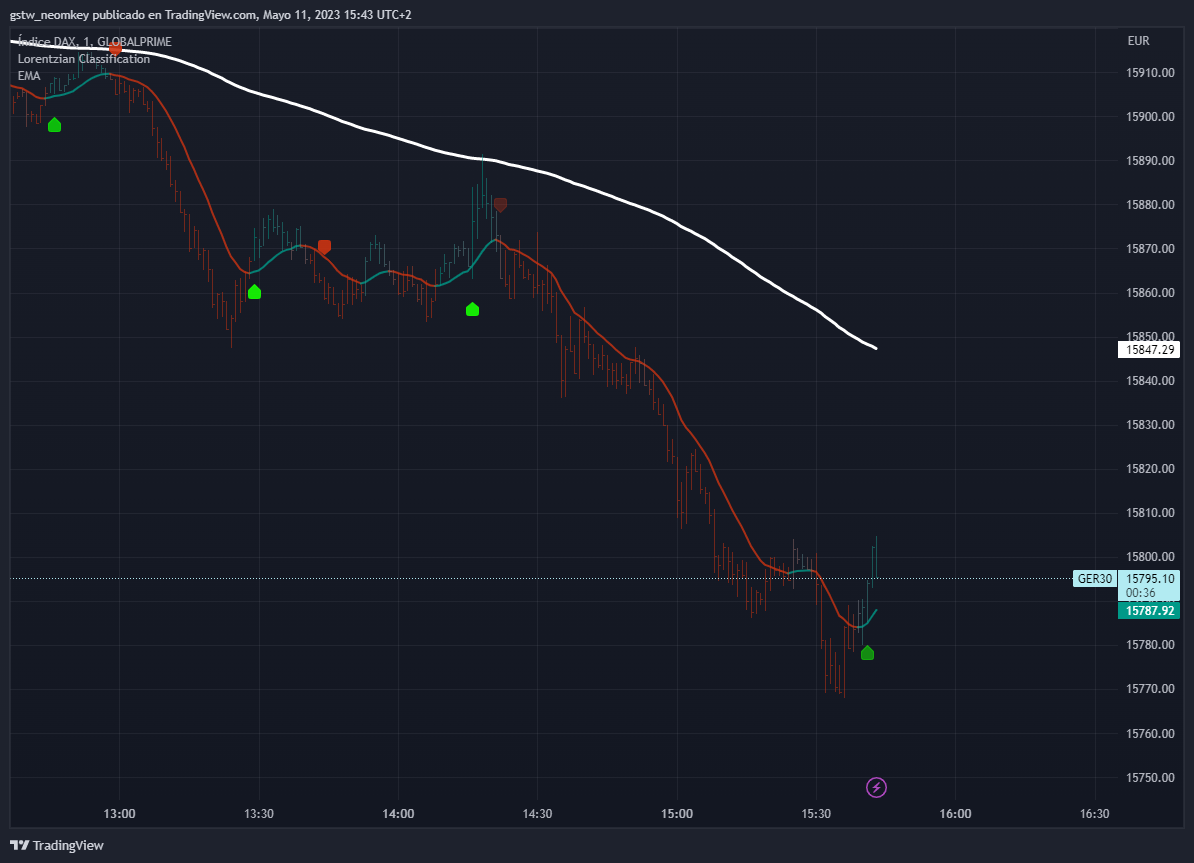
Machine Learning: Lorentzian Classification
- Forums
- Foro ProRealTime Español
- ProBuilder: Indicadores y Herramientas
- Machine Learning: Lorentzian Classification
-
AuthorPosts
-
Hola a tod@s, os dejo aquí el código y la captura de pantalla de este indicador de TRADINGVIEW, el cuál me parece bastante interesante. De este modo a ver si podría trasladar a PRT. Gracias.
// This source code is subject to the terms of the Mozilla Public License 2.0 at https://mozilla.org/MPL/2.0/ // ©jdehorty // @version=5 indicator('Machine Learning: Lorentzian Classification', 'Lorentzian Classification', true, precision=4, max_labels_count=500) import jdehorty/MLExtensions/2 as ml import jdehorty/KernelFunctions/2 as kernels // ==================== // ==== Background ==== // ==================== // When using Machine Learning algorithms like K-Nearest Neighbors, choosing an // appropriate distance metric is essential. Euclidean Distance is often used as // the default distance metric, but it may not always be the best choice. This is // because market data is often significantly impacted by proximity to significant // world events such as FOMC Meetings and Black Swan events. These major economic // events can contribute to a warping effect analogous a massive object's // gravitational warping of Space-Time. In financial markets, this warping effect // operates on a continuum, which can analogously be referred to as "Price-Time". // To help to better account for this warping effect, Lorentzian Distance can be // used as an alternative distance metric to Euclidean Distance. The geometry of // Lorentzian Space can be difficult to visualize at first, and one of the best // ways to intuitively understand it is through an example involving 2 feature // dimensions (z=2). For purposes of this example, let's assume these two features // are Relative Strength Index (RSI) and the Average Directional Index (ADX). In // reality, the optimal number of features is in the range of 3-8, but for the sake // of simplicity, we will use only 2 features in this example. // Fundamental Assumptions: // (1) We can calculate RSI and ADX for a given chart. // (2) For simplicity, values for RSI and ADX are assumed to adhere to a Gaussian // distribution in the range of 0 to 100. // (3) The most recent RSI and ADX value can be considered the origin of a coordinate // system with ADX on the x-axis and RSI on the y-axis. // Distances in Euclidean Space: // Measuring the Euclidean Distances of historical values with the most recent point // at the origin will yield a distribution that resembles Figure 1 (below). // [RSI] // | // | // | // ...:::.... // .:.:::••••••:::•::.. // .:•:.:•••::::••::••....::. // ....:••••:••••••••::••:...:•. // ...:.::::::•••:::•••:•••::.:•.. // ::•:.:•:•••••••:.:•::::::...:.. // |--------.:•••..•••••••:••:...:::•:•:..:..----------[ADX] // 0 :•:....:•••••::.:::•••::••:..... // ::....:.:••••••••:•••::••::..:. // .:...:••:::••••••••::•••....: // ::....:.....:•::•••:::::.. // ..:..::••..::::..:•:.. // .::..:::.....: // | // | // | // | // _|_ 0 // // Figure 1: Neighborhood in Euclidean Space // Distances in Lorentzian Space: // However, the same set of historical values measured using Lorentzian Distance will // yield a different distribution that resembles Figure 2 (below). // // [RSI] // ::.. | ..::: // ..... | ...... // .••••::. | :••••••. // .:•••••:. | :::••••••. // .•••••:... | .::.••••••. // .::•••••::.. | :..••••••.. // .:•••••••::.........::••••••:.. // ..::::••••.•••••••.•••••••:. // ...:•••••••.•••••••••::. // .:..••.••••••.••••.. // |---------------.:•••••••••••••••••.---------------[ADX] // 0 .:•:•••.••••••.•••••••. // .••••••••••••••••••••••••:. // .:••••••••••::..::.::••••••••:. // .::••••••::. | .::•••:::. // .:••••••.. | :••••••••. // .:••••:... | ..•••••••:. // ..:••::.. | :.•••••••. // .:•.... | ...::.:••. // ...:.. | :...:••. // :::. | ..:: // _|_ 0 // // Figure 2: Neighborhood in Lorentzian Space // Observations: // (1) In Lorentzian Space, the shortest distance between two points is not // necessarily a straight line, but rather, a geodesic curve. // (2) The warping effect of Lorentzian distance reduces the overall influence // of outliers and noise. // (3) Lorentzian Distance becomes increasingly different from Euclidean Distance // as the number of nearest neighbors used for comparison increases. // ====================== // ==== Custom Types ==== // ====================== // This section uses PineScript's new Type syntax to define important data structures // used throughout the script. type Settings float source int neighborsCount int maxBarsBack int featureCount int colorCompression bool showExits bool useDynamicExits type Label int long int short int neutral type FeatureArrays array<float> f1 array<float> f2 array<float> f3 array<float> f4 array<float> f5 type FeatureSeries float f1 float f2 float f3 float f4 float f5 type MLModel int firstBarIndex array<int> trainingLabels int loopSize float lastDistance array<float> distancesArray array<int> predictionsArray int prediction type FilterSettings bool useVolatilityFilter bool useRegimeFilter bool useAdxFilter float regimeThreshold int adxThreshold type Filter bool volatility bool regime bool adx // ========================== // ==== Helper Functions ==== // ========================== series_from(feature_string, _close, _high, _low, _hlc3, f_paramA, f_paramB) => switch feature_string "RSI" => ml.n_rsi(_close, f_paramA, f_paramB) "WT" => ml.n_wt(_hlc3, f_paramA, f_paramB) "CCI" => ml.n_cci(_close, f_paramA, f_paramB) "ADX" => ml.n_adx(_high, _low, _close, f_paramA) get_lorentzian_distance(int i, int featureCount, FeatureSeries featureSeries, FeatureArrays featureArrays) => switch featureCount 5 => math.log(1+math.abs(featureSeries.f1 - array.get(featureArrays.f1, i))) + math.log(1+math.abs(featureSeries.f2 - array.get(featureArrays.f2, i))) + math.log(1+math.abs(featureSeries.f3 - array.get(featureArrays.f3, i))) + math.log(1+math.abs(featureSeries.f4 - array.get(featureArrays.f4, i))) + math.log(1+math.abs(featureSeries.f5 - array.get(featureArrays.f5, i))) 4 => math.log(1+math.abs(featureSeries.f1 - array.get(featureArrays.f1, i))) + math.log(1+math.abs(featureSeries.f2 - array.get(featureArrays.f2, i))) + math.log(1+math.abs(featureSeries.f3 - array.get(featureArrays.f3, i))) + math.log(1+math.abs(featureSeries.f4 - array.get(featureArrays.f4, i))) 3 => math.log(1+math.abs(featureSeries.f1 - array.get(featureArrays.f1, i))) + math.log(1+math.abs(featureSeries.f2 - array.get(featureArrays.f2, i))) + math.log(1+math.abs(featureSeries.f3 - array.get(featureArrays.f3, i))) 2 => math.log(1+math.abs(featureSeries.f1 - array.get(featureArrays.f1, i))) + math.log(1+math.abs(featureSeries.f2 - array.get(featureArrays.f2, i))) // ================ // ==== Inputs ==== // ================ // Settings Object: General User-Defined Inputs Settings settings = Settings.new( input.source(title='Source', defval=close, group="General Settings", tooltip="Source of the input data"), input.int(title='Neighbors Count', defval=8, group="General Settings", minval=1, maxval=100, step=1, tooltip="Number of neighbors to consider"), input.int(title="Max Bars Back", defval=2000, group="General Settings"), input.int(title="Feature Count", defval=5, group="Feature Engineering", minval=2, maxval=5, tooltip="Number of features to use for ML predictions."), input.int(title="Color Compression", defval=1, group="General Settings", minval=1, maxval=10, tooltip="Compression factor for adjusting the intensity of the color scale."), input.bool(title="Show Default Exits", defval=false, group="General Settings", tooltip="Default exits occur exactly 4 bars after an entry signal. This corresponds to the predefined length of a trade during the model's training process.", inline="exits"), input.bool(title="Use Dynamic Exits", defval=false, group="General Settings", tooltip="Dynamic exits attempt to let profits ride by dynamically adjusting the exit threshold based on kernel regression logic.", inline="exits") ) // Trade Stats Settings // Note: The trade stats section is NOT intended to be used as a replacement for proper backtesting. It is intended to be used for calibration purposes only. showTradeStats = input.bool(true, 'Show Trade Stats', tooltip='Displays the trade stats for a given configuration. Useful for optimizing the settings in the Feature Engineering section. This should NOT replace backtesting and should be used for calibration purposes only. Early Signal Flips represent instances where the model changes signals before 4 bars elapses; high values can indicate choppy (ranging) market conditions.', group="General Settings") useWorstCase = input.bool(false, "Use Worst Case Estimates", tooltip="Whether to use the worst case scenario for backtesting. This option can be useful for creating a conservative estimate that is based on close prices only, thus avoiding the effects of intrabar repainting. This option assumes that the user does not enter when the signal first appears and instead waits for the bar to close as confirmation. On larger timeframes, this can mean entering after a large move has already occurred. Leaving this option disabled is generally better for those that use this indicator as a source of confluence and prefer estimates that demonstrate discretionary mid-bar entries. Leaving this option enabled may be more consistent with traditional backtesting results.", group="General Settings") // Settings object for user-defined settings FilterSettings filterSettings = FilterSettings.new( input.bool(title="Use Volatility Filter", defval=true, tooltip="Whether to use the volatility filter.", group="Filters"), input.bool(title="Use Regime Filter", defval=true, group="Filters", inline="regime"), input.bool(title="Use ADX Filter", defval=false, group="Filters", inline="adx"), input.float(title="Threshold", defval=-0.1, minval=-10, maxval=10, step=0.1, tooltip="Whether to use the trend detection filter. Threshold for detecting Trending/Ranging markets.", group="Filters", inline="regime"), input.int(title="Threshold", defval=20, minval=0, maxval=100, step=1, tooltip="Whether to use the ADX filter. Threshold for detecting Trending/Ranging markets.", group="Filters", inline="adx") ) // Filter object for filtering the ML predictions Filter filter = Filter.new( ml.filter_volatility(1, 10, filterSettings.useVolatilityFilter), ml.regime_filter(ohlc4, filterSettings.regimeThreshold, filterSettings.useRegimeFilter), ml.filter_adx(settings.source, 14, filterSettings.adxThreshold, filterSettings.useAdxFilter) ) // Feature Variables: User-Defined Inputs for calculating Feature Series. f1_string = input.string(title="Feature 1", options=["RSI", "WT", "CCI", "ADX"], defval="RSI", inline = "01", tooltip="The first feature to use for ML predictions.", group="Feature Engineering") f1_paramA = input.int(title="Parameter A", tooltip="The primary parameter of feature 1.", defval=14, inline = "02", group="Feature Engineering") f1_paramB = input.int(title="Parameter B", tooltip="The secondary parameter of feature 2 (if applicable).", defval=1, inline = "02", group="Feature Engineering") f2_string = input.string(title="Feature 2", options=["RSI", "WT", "CCI", "ADX"], defval="WT", inline = "03", tooltip="The second feature to use for ML predictions.", group="Feature Engineering") f2_paramA = input.int(title="Parameter A", tooltip="The primary parameter of feature 2.", defval=10, inline = "04", group="Feature Engineering") f2_paramB = input.int(title="Parameter B", tooltip="The secondary parameter of feature 2 (if applicable).", defval=11, inline = "04", group="Feature Engineering") f3_string = input.string(title="Feature 3", options=["RSI", "WT", "CCI", "ADX"], defval="CCI", inline = "05", tooltip="The third feature to use for ML predictions.", group="Feature Engineering") f3_paramA = input.int(title="Parameter A", tooltip="The primary parameter of feature 3.", defval=20, inline = "06", group="Feature Engineering") f3_paramB = input.int(title="Parameter B", tooltip="The secondary parameter of feature 3 (if applicable).", defval=1, inline = "06", group="Feature Engineering") f4_string = input.string(title="Feature 4", options=["RSI", "WT", "CCI", "ADX"], defval="ADX", inline = "07", tooltip="The fourth feature to use for ML predictions.", group="Feature Engineering") f4_paramA = input.int(title="Parameter A", tooltip="The primary parameter of feature 4.", defval=20, inline = "08", group="Feature Engineering") f4_paramB = input.int(title="Parameter B", tooltip="The secondary parameter of feature 4 (if applicable).", defval=2, inline = "08", group="Feature Engineering") f5_string = input.string(title="Feature 5", options=["RSI", "WT", "CCI", "ADX"], defval="RSI", inline = "09", tooltip="The fifth feature to use for ML predictions.", group="Feature Engineering") f5_paramA = input.int(title="Parameter A", tooltip="The primary parameter of feature 5.", defval=9, inline = "10", group="Feature Engineering") f5_paramB = input.int(title="Parameter B", tooltip="The secondary parameter of feature 5 (if applicable).", defval=1, inline = "10", group="Feature Engineering") // FeatureSeries Object: Calculated Feature Series based on Feature Variables featureSeries = FeatureSeries.new( series_from(f1_string, close, high, low, hlc3, f1_paramA, f1_paramB), // f1 series_from(f2_string, close, high, low, hlc3, f2_paramA, f2_paramB), // f2 series_from(f3_string, close, high, low, hlc3, f3_paramA, f3_paramB), // f3 series_from(f4_string, close, high, low, hlc3, f4_paramA, f4_paramB), // f4 series_from(f5_string, close, high, low, hlc3, f5_paramA, f5_paramB) // f5 ) // FeatureArrays Variables: Storage of Feature Series as Feature Arrays Optimized for ML // Note: These arrays cannot be dynamically created within the FeatureArrays Object Initialization and thus must be set-up in advance. var f1Array = array.new_float() var f2Array = array.new_float() var f3Array = array.new_float() var f4Array = array.new_float() var f5Array = array.new_float() array.push(f1Array, featureSeries.f1) array.push(f2Array, featureSeries.f2) array.push(f3Array, featureSeries.f3) array.push(f4Array, featureSeries.f4) array.push(f5Array, featureSeries.f5) // FeatureArrays Object: Storage of the calculated FeatureArrays into a single object featureArrays = FeatureArrays.new( f1Array, // f1 f2Array, // f2 f3Array, // f3 f4Array, // f4 f5Array // f5 ) // Label Object: Used for classifying historical data as training data for the ML Model Label direction = Label.new( long=1, short=-1, neutral=0 ) // Derived from General Settings maxBarsBackIndex = last_bar_index >= settings.maxBarsBack ? last_bar_index - settings.maxBarsBack : 0 // EMA Settings useEmaFilter = input.bool(title="Use EMA Filter", defval=false, group="Filters", inline="ema") emaPeriod = input.int(title="Period", defval=200, minval=1, step=1, group="Filters", inline="ema", tooltip="The period of the EMA used for the EMA Filter.") isEmaUptrend = useEmaFilter ? close > ta.ema(close, emaPeriod) : true isEmaDowntrend = useEmaFilter ? close < ta.ema(close, emaPeriod) : true useSmaFilter = input.bool(title="Use SMA Filter", defval=false, group="Filters", inline="sma") smaPeriod = input.int(title="Period", defval=200, minval=1, step=1, group="Filters", inline="sma", tooltip="The period of the SMA used for the SMA Filter.") isSmaUptrend = useSmaFilter ? close > ta.sma(close, smaPeriod) : true isSmaDowntrend = useSmaFilter ? close < ta.sma(close, smaPeriod) : true // Nadaraya-Watson Kernel Regression Settings useKernelFilter = input.bool(true, "Trade with Kernel", group="Kernel Settings", inline="kernel") showKernelEstimate = input.bool(true, "Show Kernel Estimate", group="Kernel Settings", inline="kernel") useKernelSmoothing = input.bool(false, "Enhance Kernel Smoothing", tooltip="Uses a crossover based mechanism to smoothen kernel color changes. This often results in less color transitions overall and may result in more ML entry signals being generated.", inline='1', group='Kernel Settings') h = input.int(8, 'Lookback Window', minval=3, tooltip='The number of bars used for the estimation. This is a sliding value that represents the most recent historical bars. Recommended range: 3-50', group="Kernel Settings", inline="kernel") r = input.float(8., 'Relative Weighting', step=0.25, tooltip='Relative weighting of time frames. As this value approaches zero, the longer time frames will exert more influence on the estimation. As this value approaches infinity, the behavior of the Rational Quadratic Kernel will become identical to the Gaussian kernel. Recommended range: 0.25-25', group="Kernel Settings", inline="kernel") x = input.int(25, "Regression Level", tooltip='Bar index on which to start regression. Controls how tightly fit the kernel estimate is to the data. Smaller values are a tighter fit. Larger values are a looser fit. Recommended range: 2-25', group="Kernel Settings", inline="kernel") lag = input.int(2, "Lag", tooltip="Lag for crossover detection. Lower values result in earlier crossovers. Recommended range: 1-2", inline='1', group='Kernel Settings') // Display Settings showBarColors = input.bool(true, "Show Bar Colors", tooltip="Whether to show the bar colors.", group="Display Settings") showBarPredictions = input.bool(defval = true, title = "Show Bar Prediction Values", tooltip = "Will show the ML model's evaluation of each bar as an integer.", group="Display Settings") useAtrOffset = input.bool(defval = false, title = "Use ATR Offset", tooltip = "Will use the ATR offset instead of the bar prediction offset.", group="Display Settings") barPredictionsOffset = input.float(0, "Bar Prediction Offset", minval=0, tooltip="The offset of the bar predictions as a percentage from the bar high or close.", group="Display Settings") // ================================= // ==== Next Bar Classification ==== // ================================= // This model specializes specifically in predicting the direction of price action over the course of the next 4 bars. // To avoid complications with the ML model, this value is hardcoded to 4 bars but support for other training lengths may be added in the future. src = settings.source y_train_series = src[4] < src[0] ? direction.short : src[4] > src[0] ? direction.long : direction.neutral var y_train_array = array.new_int(0) // Variables used for ML Logic var predictions = array.new_float(0) var prediction = 0. var signal = direction.neutral var distances = array.new_float(0) array.push(y_train_array, y_train_series) // ========================= // ==== Core ML Logic ==== // ========================= // Approximate Nearest Neighbors Search with Lorentzian Distance: // A novel variation of the Nearest Neighbors (NN) search algorithm that ensures a chronologically uniform distribution of neighbors. // In a traditional KNN-based approach, we would iterate through the entire dataset and calculate the distance between the current bar // and every other bar in the dataset and then sort the distances in ascending order. We would then take the first k bars and use their // labels to determine the label of the current bar. // There are several problems with this traditional KNN approach in the context of real-time calculations involving time series data: // - It is computationally expensive to iterate through the entire dataset and calculate the distance between every historical bar and // the current bar. // - Market time series data is often non-stationary, meaning that the statistical properties of the data change slightly over time. // - It is possible that the nearest neighbors are not the most informative ones, and the KNN algorithm may return poor results if the // nearest neighbors are not representative of the majority of the data. // Previously, the user @capissimo attempted to address some of these issues in several of his PineScript-based KNN implementations by: // - Using a modified KNN algorithm based on consecutive furthest neighbors to find a set of approximate "nearest" neighbors. // - Using a sliding window approach to only calculate the distance between the current bar and the most recent n bars in the dataset. // Of these two approaches, the latter is inherently limited by the fact that it only considers the most recent bars in the overall dataset. // The former approach has more potential to leverage historical price action, but is limited by: // - The possibility of a sudden "max" value throwing off the estimation // - The possibility of selecting a set of approximate neighbors that are not representative of the majority of the data by oversampling // values that are not chronologically distinct enough from one another // - The possibility of selecting too many "far" neighbors, which may result in a poor estimation of price action // To address these issues, a novel Approximate Nearest Neighbors (ANN) algorithm is used in this indicator. // In the below ANN algorithm: // 1. The algorithm iterates through the dataset in chronological order, using the modulo operator to only perform calculations every 4 bars. // This serves the dual purpose of reducing the computational overhead of the algorithm and ensuring a minimum chronological spacing // between the neighbors of at least 4 bars. // 2. A list of the k-similar neighbors is simultaneously maintained in both a predictions array and corresponding distances array. // 3. When the size of the predictions array exceeds the desired number of nearest neighbors specified in settings.neighborsCount, // the algorithm removes the first neighbor from the predictions array and the corresponding distance array. // 4. The lastDistance variable is overriden to be a distance in the lower 25% of the array. This step helps to boost overall accuracy // by ensuring subsequent newly added distance values increase at a slower rate. // 5. Lorentzian distance is used as a distance metric in order to minimize the effect of outliers and take into account the warping of // "price-time" due to proximity to significant economic events. lastDistance = -1.0 size = math.min(settings.maxBarsBack-1, array.size(y_train_array)-1) sizeLoop = math.min(settings.maxBarsBack-1, size) if bar_index >= maxBarsBackIndex //{ for i = 0 to sizeLoop //{ d = get_lorentzian_distance(i, settings.featureCount, featureSeries, featureArrays) if d >= lastDistance and i%4 //{ lastDistance := d array.push(distances, d) array.push(predictions, math.round(array.get(y_train_array, i))) if array.size(predictions) > settings.neighborsCount //{ lastDistance := array.get(distances, math.round(settings.neighborsCount*3/4)) array.shift(distances) array.shift(predictions) //} //} //} prediction := array.sum(predictions) //} // ============================ // ==== Prediction Filters ==== // ============================ // User Defined Filters: Used for adjusting the frequency of the ML Model's predictions filter_all = filter.volatility and filter.regime and filter.adx // Filtered Signal: The model's prediction of future price movement direction with user-defined filters applied signal := prediction > 0 and filter_all ? direction.long : prediction < 0 and filter_all ? direction.short : nz(signal[1]) // Bar-Count Filters: Represents strict filters based on a pre-defined holding period of 4 bars var int barsHeld = 0 barsHeld := ta.change(signal) ? 0 : barsHeld + 1 isHeldFourBars = barsHeld == 4 isHeldLessThanFourBars = 0 < barsHeld and barsHeld < 4 // Fractal Filters: Derived from relative appearances of signals in a given time series fractal/segment with a default length of 4 bars isDifferentSignalType = ta.change(signal) isEarlySignalFlip = ta.change(signal) and (ta.change(signal[1]) or ta.change(signal[2]) or ta.change(signal[3])) isBuySignal = signal == direction.long and isEmaUptrend and isSmaUptrend isSellSignal = signal == direction.short and isEmaDowntrend and isSmaDowntrend isLastSignalBuy = signal[4] == direction.long and isEmaUptrend[4] and isSmaUptrend[4] isLastSignalSell = signal[4] == direction.short and isEmaDowntrend[4] and isSmaDowntrend[4] isNewBuySignal = isBuySignal and isDifferentSignalType isNewSellSignal = isSellSignal and isDifferentSignalType // Kernel Regression Filters: Filters based on Nadaraya-Watson Kernel Regression using the Rational Quadratic Kernel // For more information on this technique refer to my other open source indicator located here: // https://www.tradingview.com/script/AWNvbPRM-Nadaraya-Watson-Rational-Quadratic-Kernel-Non-Repainting/ c_green = color.new(#009988, 20) c_red = color.new(#CC3311, 20) transparent = color.new(#000000, 100) yhat1 = kernels.rationalQuadratic(settings.source, h, r, x) yhat2 = kernels.gaussian(settings.source, h-lag, x) kernelEstimate = yhat1 // Kernel Rates of Change bool wasBearishRate = yhat1[2] > yhat1[1] bool wasBullishRate = yhat1[2] < yhat1[1] bool isBearishRate = yhat1[1] > yhat1 bool isBullishRate = yhat1[1] < yhat1 isBearishChange = isBearishRate and wasBullishRate isBullishChange = isBullishRate and wasBearishRate // Kernel Crossovers bool isBullishCrossAlert = ta.crossover(yhat2, yhat1) bool isBearishCrossAlert = ta.crossunder(yhat2, yhat1) bool isBullishSmooth = yhat2 >= yhat1 bool isBearishSmooth = yhat2 <= yhat1 // Kernel Colors color colorByCross = isBullishSmooth ? c_green : c_red color colorByRate = isBullishRate ? c_green : c_red color plotColor = showKernelEstimate ? (useKernelSmoothing ? colorByCross : colorByRate) : transparent plot(kernelEstimate, color=plotColor, linewidth=2, title="Kernel Regression Estimate") // Alert Variables bool alertBullish = useKernelSmoothing ? isBullishCrossAlert : isBullishChange bool alertBearish = useKernelSmoothing ? isBearishCrossAlert : isBearishChange // Bullish and Bearish Filters based on Kernel isBullish = useKernelFilter ? (useKernelSmoothing ? isBullishSmooth : isBullishRate) : true isBearish = useKernelFilter ? (useKernelSmoothing ? isBearishSmooth : isBearishRate) : true // =========================== // ==== Entries and Exits ==== // =========================== // Entry Conditions: Booleans for ML Model Position Entries startLongTrade = isNewBuySignal and isBullish and isEmaUptrend and isSmaUptrend startShortTrade = isNewSellSignal and isBearish and isEmaDowntrend and isSmaDowntrend // Dynamic Exit Conditions: Booleans for ML Model Position Exits based on Fractal Filters and Kernel Regression Filters lastSignalWasBullish = ta.barssince(startLongTrade) < ta.barssince(startShortTrade) lastSignalWasBearish = ta.barssince(startShortTrade) < ta.barssince(startLongTrade) barsSinceRedEntry = ta.barssince(startShortTrade) barsSinceRedExit = ta.barssince(alertBullish) barsSinceGreenEntry = ta.barssince(startLongTrade) barsSinceGreenExit = ta.barssince(alertBearish) isValidShortExit = barsSinceRedExit > barsSinceRedEntry isValidLongExit = barsSinceGreenExit > barsSinceGreenEntry endLongTradeDynamic = (isBearishChange and isValidLongExit[1]) endShortTradeDynamic = (isBullishChange and isValidShortExit[1]) // Fixed Exit Conditions: Booleans for ML Model Position Exits based on a Bar-Count Filters endLongTradeStrict = ((isHeldFourBars and isLastSignalBuy) or (isHeldLessThanFourBars and isNewSellSignal and isLastSignalBuy)) and startLongTrade[4] endShortTradeStrict = ((isHeldFourBars and isLastSignalSell) or (isHeldLessThanFourBars and isNewBuySignal and isLastSignalSell)) and startShortTrade[4] isDynamicExitValid = not useEmaFilter and not useSmaFilter and not useKernelSmoothing endLongTrade = settings.useDynamicExits and isDynamicExitValid ? endLongTradeDynamic : endLongTradeStrict endShortTrade = settings.useDynamicExits and isDynamicExitValid ? endShortTradeDynamic : endShortTradeStrict // ========================= // ==== Plotting Labels ==== // ========================= // Note: These will not repaint once the most recent bar has fully closed. By default, signals appear over the last closed bar; to override this behavior set offset=0. plotshape(startLongTrade ? low : na, 'Buy', shape.labelup, location.belowbar, color=ml.color_green(prediction), size=size.small, offset=0) plotshape(startShortTrade ? high : na, 'Sell', shape.labeldown, location.abovebar, ml.color_red(-prediction), size=size.small, offset=0) plotshape(endLongTrade and settings.showExits ? high : na, 'StopBuy', shape.xcross, location.absolute, color=#3AFF17, size=size.tiny, offset=0) plotshape(endShortTrade and settings.showExits ? low : na, 'StopSell', shape.xcross, location.absolute, color=#FD1707, size=size.tiny, offset=0) // ================ // ==== Alerts ==== // ================ // Separate Alerts for Entries and Exits alertcondition(startLongTrade, title='Open Long ▲', message='LDC Open Long ▲ | {{ticker}}@{{close}} | ({{interval}})') alertcondition(endLongTrade, title='Close Long ▲', message='LDC Close Long ▲ | {{ticker}}@{{close}} | ({{interval}})') alertcondition(startShortTrade, title='Open Short ▼', message='LDC Open Short | {{ticker}}@{{close}} | ({{interval}})') alertcondition(endShortTrade, title='Close Short ▼', message='LDC Close Short ▼ | {{ticker}}@{{close}} | ({{interval}})') // Combined Alerts for Entries and Exits alertcondition(startShortTrade or startLongTrade, title='Open Position ▲▼', message='LDC Open Position ▲▼ | {{ticker}}@{{close}} | ({{interval}})') alertcondition(endShortTrade or endLongTrade, title='Close Position ▲▼', message='LDC Close Position ▲▼ | {{ticker}}@[{{close}}] | ({{interval}})') // Kernel Estimate Alerts alertcondition(condition=alertBullish, title='Kernel Bullish Color Change', message='LDC Kernel Bullish ▲ | {{ticker}}@{{close}} | ({{interval}})') alertcondition(condition=alertBearish, title='Kernel Bearish Color Change', message='LDC Kernel Bearish ▼ | {{ticker}}@{{close}} | ({{interval}})') // ========================= // ==== Display Signals ==== // ========================= atrSpaced = useAtrOffset ? ta.atr(1) : na compressionFactor = settings.neighborsCount / settings.colorCompression c_pred = prediction > 0 ? color.from_gradient(prediction, 0, compressionFactor, #787b86, #009988) : prediction <= 0 ? color.from_gradient(prediction, -compressionFactor, 0, #CC3311, #787b86) : na c_label = showBarPredictions ? c_pred : na c_bars = showBarColors ? color.new(c_pred, 50) : na x_val = bar_index y_val = useAtrOffset ? prediction > 0 ? high + atrSpaced: low - atrSpaced : prediction > 0 ? high + hl2*barPredictionsOffset/20 : low - hl2*barPredictionsOffset/30 label.new(x_val, y_val, str.tostring(prediction), xloc.bar_index, yloc.price, color.new(color.white, 100), label.style_label_up, c_label, size.normal, text.align_left) barcolor(showBarColors ? color.new(c_pred, 50) : na) // ===================== // ==== Backtesting ==== // ===================== // The following can be used to stream signals to a backtest adapter backTestStream = switch startLongTrade => 1 endLongTrade => 2 startShortTrade => -1 endShortTrade => -2 plot(backTestStream, "Backtest Stream", display=display.none) // The following can be used to display real-time trade stats. This can be a useful mechanism for obtaining real-time feedback during Feature Engineering. This does NOT replace the need to properly backtest. // Note: In this context, a "Stop-Loss" is defined instances where the ML Signal prematurely flips directions before an exit signal can be generated. [totalWins, totalLosses, totalEarlySignalFlips, totalTrades, tradeStatsHeader, winLossRatio, winRate] = ml.backtest(high, low, open, startLongTrade, endLongTrade, startShortTrade, endShortTrade, isEarlySignalFlip, maxBarsBackIndex, bar_index, settings.source, useWorstCase) init_table() => c_transparent = color.new(color.black, 100) table.new(position.top_right, columns=2, rows=7, frame_color=color.new(color.black, 100), frame_width=1, border_width=1, border_color=c_transparent) update_table(tbl, tradeStatsHeader, totalTrades, totalWins, totalLosses, winLossRatio, winRate, stopLosses) => c_transparent = color.new(color.black, 100) table.cell(tbl, 0, 0, tradeStatsHeader, text_halign=text.align_center, text_color=color.gray, text_size=size.normal) table.cell(tbl, 0, 1, 'Winrate', text_halign=text.align_center, bgcolor=c_transparent, text_color=color.gray, text_size=size.normal) table.cell(tbl, 1, 1, str.tostring(totalWins / totalTrades, '#.#%'), text_halign=text.align_center, bgcolor=c_transparent, text_color=color.gray, text_size=size.normal) table.cell(tbl, 0, 2, 'Trades', text_halign=text.align_center, bgcolor=c_transparent, text_color=color.gray, text_size=size.normal) table.cell(tbl, 1, 2, str.tostring(totalTrades, '#') + ' (' + str.tostring(totalWins, '#') + '|' + str.tostring(totalLosses, '#') + ')', text_halign=text.align_center, bgcolor=c_transparent, text_color=color.gray, text_size=size.normal) table.cell(tbl, 0, 5, 'WL Ratio', text_halign=text.align_center, bgcolor=c_transparent, text_color=color.gray, text_size=size.normal) table.cell(tbl, 1, 5, str.tostring(totalWins / totalLosses, '0.00'), text_halign=text.align_center, bgcolor=c_transparent, text_color=color.gray, text_size=size.normal) table.cell(tbl, 0, 6, 'Early Signal Flips', text_halign=text.align_center, bgcolor=c_transparent, text_color=color.gray, text_size=size.normal) table.cell(tbl, 1, 6, str.tostring(totalEarlySignalFlips, '#'), text_halign=text.align_center, bgcolor=c_transparent, text_color=color.gray, text_size=size.normal) if showTradeStats var tbl = ml.init_table() if barstate.islast update_table(tbl, tradeStatsHeader, totalTrades, totalWins, totalLosses, winLossRatio, winRate, totalEarlySignalFlips)Bien, ese es otro promedio móvil (un promedio móvil de mínimos cuadrados pero no con una distancia euclidiana, sino con una distancia lorentziana). Por qué no, pero le aseguro que no obtendrá algo más significativo al final que un MA de regresión lineal. Una parte del código está ofuscado porque está ubicado en funciones externas (el código fuente no está completo):
importar jdehorty / MLExtensions / 2 como mlimportar jdehorty / KernelFunctions / 2 como núcleosthanked this postMuchísimas gracias Nicolás por responder. Realizaré una comparación con los datos aportados con una MA de Regresión Lineal.
Un saludo.
Hola Neo
Algo que funciona de maravilla iniciado por Nicolas
// LINEAR REGRESSION CHANNEL V2 by Nicolas
// echelle lineaire//PRC_Std and Ste LinRegChannel indicator //Standard Deviation and Standard Error
//Linear Regression Channel //12.03.2019
//Nicolas @ http://www.prorealcode.com //Sharing ProRealTime knowledgedefparam drawonlastbaronly= true
if islastbarupdate then
// — settings
lookback= max(1,barindex) //channel period
ChannelType = 1 //1= Standard Deviation ; 2= Standard Erro
NbDeviation = 1 //Deviation multiplier
NbDeviation2 = 0.5 //Deviation multiplier
colorRed = 255
colorGreen = 255
colorBlue = 0
// — end of settingssumx = 0
sumy = 0
sumxy = 0
sumx2 = 0for cmpt = lookback downto 0 do
tmpx = cmpt
tmpy = close[cmpt]
sumy = sumy+tmpy
sumx = sumx+tmpx
sumx2 = sumx2 + (tmpx*tmpx)
sumxy = sumxy + (tmpy*tmpx)
nextn = lookback+1
if (sumx2 = sumx * sumx) then // protection to avoid infinite values
b = sumxy – sumx * sumy
else
b = (n * sumxy – sumx * sumy) / (n * sumx2 – sumx * sumx)
endif
a = (sumy – b * sumx) / ndrawsegment(barindex[lookback],a+b*lookback,barindex,a+b*0) coloured(“white”)style(line,5)
//channel
if ChannelType = 1 then //Standard Deviation
dat = std[lookback]*NbDeviation
dat2 = std[lookback]*NbDeviation2
dat3 = std[lookback]*NbDeviation3
else
dat = ste[lookback]*NbDeviation
dat2 = ste[lookback]*NbDeviation2
dat3 = ste[lookback]*NbDeviation3
endif
drawsegment(barindex[lookback],(a+b*lookback)+dat,barindex,a+b*0+dat) coloured(“red”) style(line,2)
drawsegment(barindex[lookback],(a+b*lookback)-dat,barindex,a+b*0-dat) coloured(“green”) style(line,2)
drawsegment(barindex[lookback],(a+b*lookback)+dat2,barindex,a+b*0+dat2) coloured(“yellow”) style(line,3)
drawsegment(barindex[lookback],(a+b*lookback)-dat2,barindex,a+b*0-dat2) coloured(“yellow”) style(line,3)
endif
/////////////////////////////////////////////////////////////////////////////
NbDeviation3 = 1.5 //Deviation multiplier
drawsegment(barindex[lookback],(a+b*lookback)+dat3,barindex,a+b*0+dat3) coloured(“red”) style(dottedline,3)
drawsegment(barindex[lookback],(a+b*lookback)-dat3,barindex,a+b*0-dat3) coloured(“green”) style(dottedline,3)
////////////////////////////////////////////////////////////////////////////////
return customclose as ” LINEAR REGRESSION CHANNEL V2 “thanked this postgrafico del IBEX35
Hola Supertiti,
muchas gracias por el aporte, voy a probar a ver qué tal.
Un saludo
Buenos días a todos, me preguntaba cómo iba todo esto. Yo también noté este indicador en TradingView y estoy interesado en saber si se puede utilizar en PRT…
Hola Mitchy14 Estoy intentando crear alertas con esa estrategia para que cuando me pinte los indicadores flecha verde arriba y flecha roja abajo me lance las alertas correspondientes pero TradingView no dispara las alertas Me pueden ayudar a configurar trandigView ? GraciasLo sentimos, pero este foro está dedicado únicamente a la plataforma ProRealTime. Encontrará otros foros en Internet sobre diferentes plataformas comerciales.Good morning all, sadly I dont speak Spanish and my auto translate is giving me strange results. In short – I have been trying to re-write this without the pine script, it would be great if someone could confirm whether the following works / looks as intended:Buenos días a todos. Lamentablemente, no hablo español y mi traductor automático me da resultados extraños. En resumen, he estado intentando reescribir esto sin el script de Pine. Sería genial si alguien pudiera confirmar si lo siguiente funciona o se ve como se espera:
// ============================================================
// Machine Learning: Lorentzian Classification for ProRealTime
// Converted from TradingView PineScript (©jdehorty)
// ============================================================
// ProBuilder adaptation preserving core ML algorithm.
// ============================================================
// === SETTINGS ===
DEFPARAM CalculateOnLastBars = 2000
// General Settings
neighborsCount = 8
maxBarsBack = 2000
featureCount = 5
// Feature Engineering Settings
// Feature 1: RSI
f1paramA = 14
// Feature 2: WT (Wave Trend approximation)
f2paramA = 10
f2paramB = 11
// Feature 3: CCI
f3paramA = 20
// Feature 4: ADX
f4paramA = 20
// Feature 5: RSI (second instance)
f5paramA = 9
// Filter Settings
useVolatilityFilter = 1
useRegimeFilter = 1
useAdxFilter = 0
adxThreshold = 20
regimeThreshold = -0.1
useEmaFilter = 0
emaPeriod = 200
useSmaFilter = 0
smaPeriod = 200
// Kernel Settings
useKernelFilter = 1
showKernelEstimate = 1
useKernelSmoothing = 0
hh = 8
rr = 8.0
xx = 25
lag = 2
// Display Settings
showExits = 0
// ============================================================
// === FEATURE CALCULATIONS ===
// ============================================================
// Feature 1: Normalized RSI
myRSI1 = RSI[f1paramA](close)
f1 = (myRSI1 – 50) / 50
// Feature 2: Normalized Wave Trend (approximation)
ap2 = (high + low + close) / 3
esa2 = ExponentialAverage[f2paramA](ap2)
d2 = ExponentialAverage[f2paramA](abs(ap2 – esa2))
IF d2 <> 0 THEN
ci2 = (ap2 – esa2) / (0.015 * d2)
ELSE
ci2 = 0
ENDIF
wt1 = ExponentialAverage[f2paramB](ci2)
f2 = wt1 / 100
// Feature 3: Normalized CCI
myCCI = CCI[f3paramA](close)
f3 = myCCI / 200
// Feature 4: Normalized ADX
myADX = ADX[f4paramA]
f4 = (myADX – 25) / 25
// Feature 5: Normalized RSI (second)
myRSI2 = RSI[f5paramA](close)
f5 = (myRSI2 – 50) / 50
// ============================================================
// === TRAINING LABELS (Next 4-bar classification) ===
// ============================================================
src = close
IF src[4] < src[0] THEN
yTrain = -1
ELSIF src[4] > src[0] THEN
yTrain = 1
ELSE
yTrain = 0
ENDIF
// ============================================================
// === FILTER CALCULATIONS ===
// ============================================================
// Volatility Filter
IF useVolatilityFilter THEN
recentAtr = AverageTrueRange[1](close)
historicalAtr = AverageTrueRange[10](close)
IF historicalAtr <> 0 THEN
isNotAdverseVol = (recentAtr <= historicalAtr * 1.0)
ELSE
isNotAdverseVol = 1
ENDIF
ELSE
isNotAdverseVol = 1
ENDIF
// Regime Filter
IF useRegimeFilter THEN
regimeSlope = LinearRegression[10](close) – LinearRegression[10](close)[1]
isRegimeOK = (regimeSlope > regimeThreshold)
ELSE
isRegimeOK = 1
ENDIF
// ADX Filter
IF useAdxFilter THEN
filterADX = ADX[14]
isAdxOK = (filterADX > adxThreshold)
ELSE
isAdxOK = 1
ENDIF
// EMA Filter
IF useEmaFilter THEN
myEma = ExponentialAverage[emaPeriod](close)
isEmaUptrend = (close > myEma)
isEmaDowntrend = (close < myEma)
ELSE
isEmaUptrend = 1
isEmaDowntrend = 1
ENDIF
// SMA Filter
IF useSmaFilter THEN
mySma = Average[smaPeriod](close)
isSmaUptrend = (close > mySma)
isSmaDowntrend = (close < mySma)
ELSE
isSmaUptrend = 1
isSmaDowntrend = 1
ENDIF
// Combined filter
filterAll = isNotAdverseVol AND isRegimeOK AND isAdxOK
// ============================================================
// === CORE ML LOGIC: Approximate Nearest Neighbors ===
// === with Lorentzian Distance ===
// ============================================================
lastDistance = -1.0
size = min(maxBarsBack – 1, BarIndex – 1)
sizeLoop = min(maxBarsBack – 1, size)
distCount = 0
FOR i = 0 TO sizeLoop
// Calculate Lorentzian Distance
IF featureCount >= 5 THEN
d = log(1 + abs(f1 – f1[i])) + log(1 + abs(f2 – f2[i])) + log(1 + abs(f3 – f3[i])) + log(1 + abs(f4 – f4[i])) + log(1 + abs(f5 – f5[i]))
ELSIF featureCount = 4 THEN
d = log(1 + abs(f1 – f1[i])) + log(1 + abs(f2 – f2[i])) + log(1 + abs(f3 – f3[i])) + log(1 + abs(f4 – f4[i]))
ELSIF featureCount = 3 THEN
d = log(1 + abs(f1 – f1[i])) + log(1 + abs(f2 – f2[i])) + log(1 + abs(f3 – f3[i]))
ELSE
d = log(1 + abs(f1 – f1[i])) + log(1 + abs(f2 – f2[i]))
ENDIF
// Only consider every 4th bar and distances >= lastDistance
IF d >= lastDistance AND (i MOD 4) <> 0 THEN
lastDistance = d
distCount = distCount + 1
$distances[distCount] = d
$predictions[distCount] = round(yTrain[i])
// Trim to neighborsCount
IF distCount > neighborsCount THEN
trimIdx = round(neighborsCount * 3 / 4)
IF trimIdx >= 1 AND trimIdx <= distCount THEN
lastDistance = $distances[trimIdx]
ENDIF
FOR j = 1 TO distCount – 1
$distances[j] = $distances[j + 1]
$predictions[j] = $predictions[j + 1]
NEXT
distCount = distCount – 1
ENDIF
ENDIF
NEXT
// Sum predictions
predictionSum = 0
FOR k = 1 TO distCount
predictionSum = predictionSum + $predictions[k]
NEXT
prediction = predictionSum
// ============================================================
// === NADARAYA-WATSON KERNEL REGRESSION ===
// ============================================================
// Rational Quadratic Kernel
yhat1 = 0
sumWeights1 = 0
FOR i = 0 TO hh – 1
w1 = pow(1 + (pow(i, 2) / (2 * rr * pow(xx, 2))), -rr)
yhat1 = yhat1 + w1 * close[i]
sumWeights1 = sumWeights1 + w1
NEXT
IF sumWeights1 <> 0 THEN
yhat1 = yhat1 / sumWeights1
ENDIF
// Gaussian Kernel
yhat2 = 0
sumWeights2 = 0
gaussH = max(1, hh – lag)
FOR i = 0 TO gaussH – 1
w2 = exp(-pow(i, 2) / (2 * pow(xx, 2)))
yhat2 = yhat2 + w2 * close[i]
sumWeights2 = sumWeights2 + w2
NEXT
IF sumWeights2 <> 0 THEN
yhat2 = yhat2 / sumWeights2
ENDIF
kernelEstimate = yhat1
// Kernel Rates of Change
wasBearishRate = (yhat1[2] > yhat1[1])
wasBullishRate = (yhat1[2] < yhat1[1])
isBearishRate = (yhat1[1] > yhat1)
isBullishRate = (yhat1[1] < yhat1)
isBearishChange = isBearishRate AND wasBullishRate
isBullishChange = isBullishRate AND wasBearishRate
// Kernel Crossovers
isBullishCross = (yhat2 >= yhat1 AND yhat2[1] < yhat1[1])
isBearishCross = (yhat2 <= yhat1 AND yhat2[1] > yhat1[1])
isBullishSmooth = (yhat2 >= yhat1)
isBearishSmooth = (yhat2 <= yhat1)
// Kernel filter booleans
IF useKernelSmoothing THEN
alertBullish = isBullishCross
alertBearish = isBearishCross
ELSE
alertBullish = isBullishChange
alertBearish = isBearishChange
ENDIF
IF useKernelFilter THEN
IF useKernelSmoothing THEN
isBullish = isBullishSmooth
isBearish = isBearishSmooth
ELSE
isBullish = isBullishRate
isBearish = isBearishRate
ENDIF
ELSE
isBullish = 1
isBearish = 1
ENDIF
// ============================================================
// === SIGNAL GENERATION ===
// ============================================================
// Filtered signal
IF prediction > 0 AND filterAll THEN
signal = 1
ELSIF prediction < 0 AND filterAll THEN
signal = -1
ELSE
signal = signal[1]
ENDIF
// Detect signal changes
isDiffSignal = (signal <> signal[1])
// Buy/Sell conditions
isBuySignal = (signal = 1 AND isEmaUptrend AND isSmaUptrend)
isSellSignal = (signal = -1 AND isEmaDowntrend AND isSmaDowntrend)
isNewBuySignal = (isBuySignal AND isDiffSignal)
isNewSellSignal = (isSellSignal AND isDiffSignal)
// Entry Conditions
startLong = (isNewBuySignal AND isBullish)
startShort = (isNewSellSignal AND isBearish)
// Exit Conditions (strict 4-bar hold)
IF startLong OR startShort THEN
barsHeld = 0
ELSE
barsHeld = barsHeld[1] + 1
ENDIF
isHeldFourBars = (barsHeld = 4)
endLong = (isHeldFourBars AND signal[4] = 1)
endShort = (isHeldFourBars AND signal[4] = -1)
// ============================================================
// === DISPLAY ===
// ============================================================
atr = AverageTrueRange[10](close) * 0.5
// Plot Buy/Sell signals
IF startLong THEN
DRAWARROWUP(barindex, low – atr) COLOURED(0, 153, 0)
DRAWTEXT(“BUY”, barindex, low – atr * 2, Dialog, Bold, 10) COLOURED(0, 153, 0)
ENDIF
IF startShort THEN
DRAWARROWDOWN(barindex, high + atr) COLOURED(204, 51, 17)
DRAWTEXT(“SELL”, barindex, high + atr * 2, Dialog, Bold, 10) COLOURED(204, 51, 17)
ENDIF
// Plot Exits
IF showExits AND endLong THEN
DRAWTEXT(“X”, barindex, high + atr, Dialog, Bold, 12) COLOURED(58, 255, 23)
ENDIF
IF showExits AND endShort THEN
DRAWTEXT(“X”, barindex, low – atr, Dialog, Bold, 12) COLOURED(253, 23, 7)
ENDIF
// === DISPLAY ===
atr = AverageTrueRange[10](close) * 0.5
// Plot Buy/Sell signals
IF startLong THEN
DRAWARROWUP(barindex, low – atr) COLOURED(0,153,0)
DRAWTEXT(“BUY”, barindex, low – atr * 2, Dialog, Bold, 10) COLOURED(0,153,0)
ENDIF
IF startShort THEN
DRAWARROWDOWN(barindex, high + atr) COLOURED(204,51,17)
DRAWTEXT(“SELL”, barindex, high + atr * 2, Dialog, Bold, 10) COLOURED(204,51,17)
ENDIF
// Plot Exits
IF showExits AND endLong THEN
DRAWTEXT(“X”, barindex, high + atr, Dialog, Bold, 12) COLOURED(58,255,23)
ENDIF
IF showExits AND endShort THEN
DRAWTEXT(“X”, barindex, low – atr, Dialog, Bold, 12) COLOURED(253,23,7)
ENDIF
// Choose color for kernel line
IF isBullishRate THEN
kernelColorR = 0
kernelColorG = 153
kernelColorB = 136
ELSE
kernelColorR = 204
kernelColorG = 51
kernelColorB = 17
ENDIF
// *** FINAL LINE – NOTHING AFTER THIS ***
RETURN kernelEstimate COLOURED(kernelColorR,kernelColorG,kernelColorB) AS “Kernel”
Puedes escribir en este grupo si necesitas traducir algún código de tradingview a prorealtime
TradingView to ProRealTime Translation Center
@Roq
Por favor, usa solo el idioma del foro elegido. Si no hablas ese idioma o no encuentras un traductor, abre un nuevo tema en el idioma que prefieras.
Gracias 🙂
-
AuthorPosts
- You must be logged in to reply to this topic.
Machine Learning: Lorentzian Classification
ProBuilder: Indicadores y Herramientas
Author
Summary
This topic contains 11 replies,
has 3 voices, and was last updated by ![]() robertogozzi
robertogozzi
1 month, 3 weeks ago.
Topic Details
| Forum: | ProBuilder: Indicadores y Herramientas |
| Language: | Spanish |
| Started: | 05/11/2023 |
| Status: | Active |
| Attachments: | 2 files |
About personal data collected
The information collected on this form is stored in a computer file by ProRealCode to create and access your ProRealCode profile. This data is kept in a secure database for the duration of the member's membership. They will be kept as long as you use our services and will be automatically deleted after 3 years of inactivity. Your personal data is used to create your private profile on ProRealCode. This data is maintained by SAS ProRealCode, 407 rue Freycinet, 59151 Arleux, France. If you subscribe to our newsletters, your email address is provided to our service provider "MailChimp" located in the United States, with whom we have signed a confidentiality agreement. This company is also compliant with the EU/Swiss Privacy Shield, and the GDPR. For any request for correction or deletion concerning your data, you can directly contact the ProRealCode team by email at privacy@prorealcode.com If you would like to lodge a complaint regarding the use of your personal data, you can contact your data protection supervisory authority.