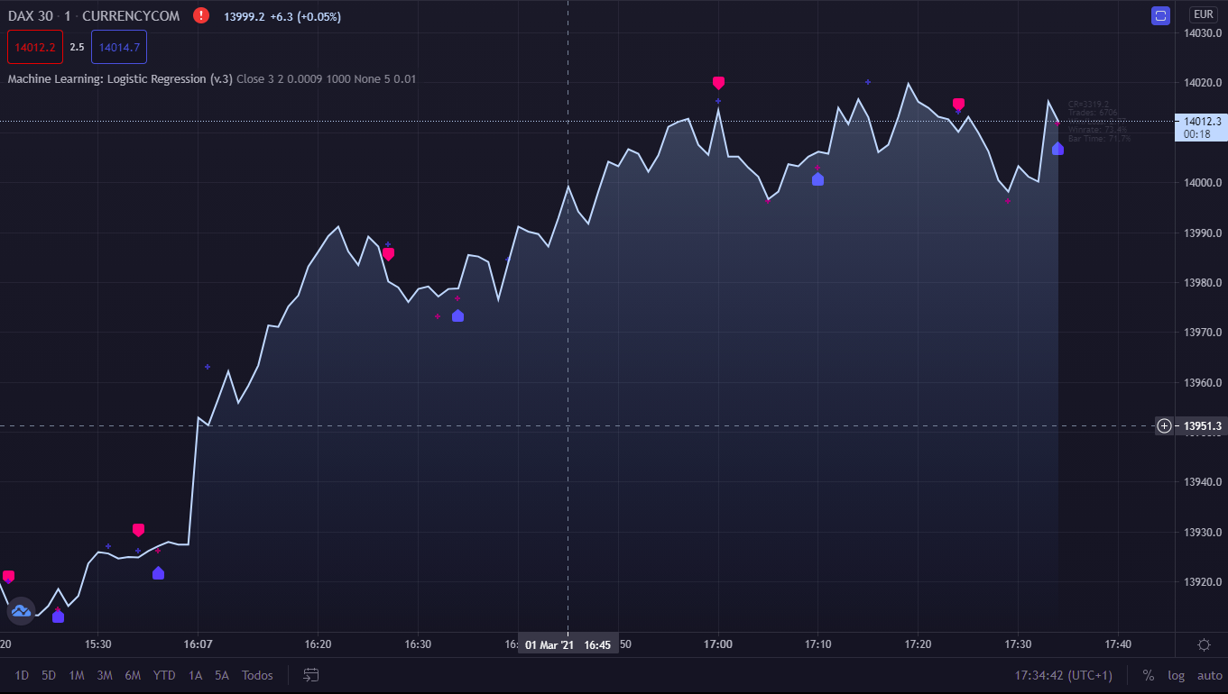
Hola a todos, me gustaría poder tener este indicador (proveniente de la plataforma Tradingview) en PRT v.11.

Os dejo el código, así cómo un pantallazo de dicho indicador en Tradingview.
Muchas gracias de antemano.

————————————————————————————————————————————

// This source code is subject to the terms of the Mozilla Public License 2.0 at https://mozilla.org/MPL/2.0/
// © capissimo

//@version=4
study(‘Machine Learning: Logistic Regression (v.3)’, ”, true)

// Multi-timeframe Strategy based on Logistic Regression algorithm

// Description:

// This strategy uses a classic machine learning algorithm that came from statistics –
// Logistic Regression (LR).

// The first and most important thing about logistic regression is that it is not a
// ‘Regression’ but a ‘Classification’ algorithm. The name itself is somewhat misleading.
// Regression gives a continuous numeric output but most of the time we need the output in
// classes (i.e. categorical, discrete). For example, we want to classify emails into “spam” or
// ‘not spam’, classify treatment into “success” or ‘failure’, classify statement into “right”
// or ‘wrong’, classify election data into ‘fraudulent vote’ or ‘non-fraudulent vote’,
// classify market move into ‘long’ or ‘short’ and so on. These are the examples of
// logistic regression having a binary output (also called dichotomous).

// You can also think of logistic regression as a special case of linear regression when the
// outcome variable is categorical, where we are using log of odds as dependent variable.
// In simple words, it predicts the probability of occurrence of an event by fitting data to a
// logit function.

// Basically, the theory behind Logistic Regression is very similar to the one from Linear
// Regression, where we seek to draw a best-fitting line over data points, but in Logistic
// Regression, we don’t directly fit a straight line to our data like in linear regression.
// Instead, we fit a S shaped curve, called Sigmoid, to our observations, that best
// SEPARATES data points. Technically speaking, the main goal of building the model is to
// find the parameters (weights) using gradient descent.

// In this script the LR algorithm is retrained on each new bar trying to classify it
// into one of the two categories. This is done via the logistic_regression function by
// updating the weights w in the loop that continues for iterations number of times.
// In the end the weights are passed through the sigmoid function, yielding a
// prediction.

// Mind that some assets require to modify the script’s input parameters. For instance,
// when used with BTCUSD and USDJPY, the ‘Normalization Lookback’ parameter should be set
// down to 4 (2,…,5..), and optionally the ‘Use Price Data for Signal Generation?’
// parameter should be checked. The defaults were tested with EURUSD.

// Note: TradingViews’s playback feature helps to see this strategy in action.
// Warning: Signals ARE repainting.

// Style tags: Trend Following, Trend Analysis
// Asset class: Equities, Futures, ETFs, Currencies and Commodities
// Dataset: FX Minutes/Hours++/Days

//——————– Inputs

ptype = input(‘Close’,’Price Type’, options=[‘Open’,’High’,’Low’,’Close’,’HL2′,’OC2′,’OHL3′,’HLC3′,’OHLC4′])
reso = input(”, ‘Resolution’, input.resolution)
lookback = input(3, ‘Lookback Window Size |2..n| (2)’, minval=2)
nlbk = input(2, ‘Normalization Lookback |2..240| (120)’, minval=2, maxval=240)
lrate = input(0.0009, ‘Learning Rate |0.0001..0.01|’, minval=0.0001, maxval=0.01, step=0.0001)
iterations = input(1000, ‘Training Iterations |50..20000|’, minval=50)
ftype = input(‘None’, ‘Filter Signals by’, options=[‘Volatility’,’Volume’,’Both’,’None’])
curves = input(false, ‘Show Loss & Prediction Curves?’)
easteregg = input(true, ‘Optional Calculation?’)
useprice = input(true, ‘Use Price Data for Signal Generation?’)
holding_p = input(5, ‘Holding Period |1..n|’, minval=1)

//——————– System Variables

var BUY = 1, var SELL = -1, var HOLD = 0
var signal = HOLD
var hp_counter = 0

//——————– Custom Functions

cAqua(g) => g>9?#0080FFff:g>8?#0080FFe5:g>7?#0080FFcc:g>6?#0080FFb2:g>5?#0080FF99
: g>4?#0080FF7f:g>3?#0080FF66:g>2?#0080FF4c:g>1?#0080FF33:#00C0FF19
cPink(g) => g>9?#FF0080ff:g>8?#FF0080e5:g>7?#FF0080cc:g>6?#FF0080b2:g>5?#FF008099
: g>4?#FF00807f:g>3?#FF008066:g>2?#FF00804c:g>1?#FF008033:#FF008019

volumeBreak(thres) =>
rsivol = rsi(volume, 14)
osc = hma(rsivol, 10)
osc > thres

volatilityBreak(volmin, volmax) => atr(volmin) > atr(volmax)

dot(v, w, p) => sum(v * w, p) // dot product

sigmoid(z) => 1.0 / (1.0 + exp(-z))

logistic_regression(X, Y, p, lr, iterations) =>
w = 0.0, loss = 0.0
for i=1 to iterations
hypothesis = sigmoid(dot(X, 0.0, p)) //– prediction
loss := -1.0 / p * (dot(dot(Y, log(hypothesis) + (1.0 – Y), p), log(1.0 – hypothesis), p))
gradient = 1.0 / p * (dot(X, hypothesis – Y, p))
w := w – lr * gradient //– update weights

[loss, sigmoid(dot(X, w, p))] //– current loss & prediction

minimax(ds, p, min, max) => // normalize to price
hi = highest(ds, p), lo = lowest(ds, p)
(max – min) * (ds – lo)/(hi – lo) + min

//——————– Logic

ds = ptype==’Open’ ? open
: ptype==’High’ ? high
: ptype==’Low’ ? low
: ptype==’Close’ ? close
: ptype==’HL2′ ? (high+low)/2
: ptype==’OC2′ ? (open+close)/2
: ptype==’OHL3′ ? (open+high+low)/3
: ptype==’HLC3′ ? (high+low+close)/3
: (open+high+low+close)/4

base_ds = security(”, reso, ds[barstate.ishistory ? 0 : 1])
synth_ds = log(abs(pow(base_ds, 2) – 1) + .5) //– generate a synthetic dataset

base = easteregg ? time : base_ds //– standard and optional calculation
synth = easteregg ? base_ds : synth_ds

[loss, prediction] = logistic_regression(base, synth, lookback, lrate, iterations)
scaled_loss = minimax(loss, nlbk, lowest(base_ds, nlbk), highest(base_ds, nlbk))
scaled_prediction = minimax(prediction, nlbk, lowest(base_ds, nlbk), highest(base_ds, nlbk))

filter = ftype==’Volatility’ ? volatilityBreak(1, 10)
: ftype==’Volume’ ? volumeBreak(49)
: ftype==’Both’ ? volatilityBreak(1, 10) and volumeBreak(49)
: true

signal := useprice ?
base_ds < scaled_loss and filter ? SELL : base_ds > scaled_loss and filter ? BUY : nz(signal[1])
: crossunder(scaled_loss, scaled_prediction) and filter ? SELL : crossover(scaled_loss, scaled_prediction) and filter ? BUY : nz(signal[1])

changed = change(signal)

hp_counter := changed ? 0 : hp_counter + 1

startLongTrade = changed and signal==BUY
startShortTrade = changed and signal==SELL
endLongTrade = (signal==BUY and hp_counter==holding_p and not changed) or (changed and signal==SELL)
endShortTrade = (signal==SELL and hp_counter==holding_p and not changed) or (changed and signal==BUY)

//——————– Rendering

plot(curves ? scaled_loss : na, ”, color.blue, 3)
plot(curves ? scaled_prediction : na, ”, color.lime, 3)

plotshape(startLongTrade ? low : na, ‘Buy’, shape.labelup, location.belowbar, cAqua(10), size=size.small)
plotshape(startShortTrade ? high : na, ‘Sell’, shape.labeldown, location.abovebar, cPink(10), size=size.small)
plot(endLongTrade ? high : na, ‘StopBuy’, cAqua(6), 2, plot.style_cross)
plot(endShortTrade ? low : na, ‘StopSell’, cPink(6), 2, plot.style_cross)

//——————– Alerting

alertcondition(startLongTrade, ‘Buy’, ‘Go long!’)
alertcondition(startShortTrade, ‘Sell’, ‘Go short!’)
alertcondition(startLongTrade or startShortTrade, ‘Alert’, ‘Deal Time!’) //– general alert

//——————– Backtesting (TODO)

lot_size = input(0.01, ‘Lot Size’, options=[0.01,0.1,0.2,0.3,0.5,1,2,3,5,10,20,30,50,100,1000])

ohl3 = (open+high+low)/3

var float start_long_trade = 0.
var float long_trades = 0.
var float start_short_trade = 0.
var float short_trades = 0.
var int wins = 0
var int trade_count = 0

if startLongTrade
start_long_trade := ohl3
if endLongTrade
trade_count := 1
ldiff = (ohl3 – start_long_trade)
wins := ldiff > 0 ? 1 : 0
long_trades := ldiff * lot_size
if startShortTrade
start_short_trade := ohl3
if endShortTrade
trade_count := 1
sdiff = (start_short_trade – ohl3)
wins := sdiff > 0 ? 1 : 0
short_trades := sdiff * lot_size

cumreturn = cum(long_trades) + cum(short_trades) //– cumulative return
totaltrades = cum(trade_count)
totalwins = cum(wins)
totallosses = totaltrades – totalwins == 0 ? 1 : totaltrades – totalwins

//——————– Information

show_info = input(true, ‘Show Info?’)

var label lbl = na

tbase = (time – time[1]) / 1000
tcurr = (timenow – time_close[1]) / 1000

info = ‘CR=’ + tostring(cumreturn, ‘#.#’)
+ ‘\nTrades: ‘ + tostring(totaltrades, ‘#’)
+ ‘\nWin/Loss: ‘ + tostring(totalwins/totallosses, ‘#.##’)
+ ‘\nWinrate: ‘ + tostring(totalwins/totaltrades, ‘#.#%’)
+ ‘\nBar Time: ‘ + tostring(tcurr / tbase, ‘#.#%’)

if show_info and barstate.islast
lbl := label.new(bar_index, close, info, xloc.bar_index, yloc.price,
color.new(color.blue, 100), label.style_label_left, color.black, size.small, text.align_left)
label.delete(lbl[1])

Preview-TradingviewIndicator.png