All,

I have modified the "Quino Statistics Plotter" indicator created last August,
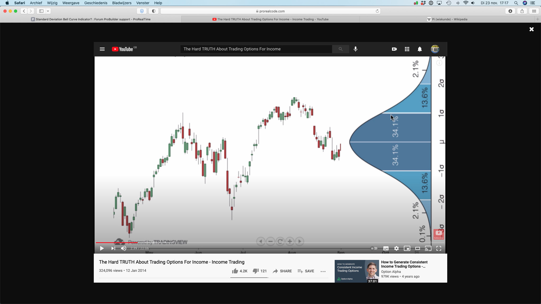
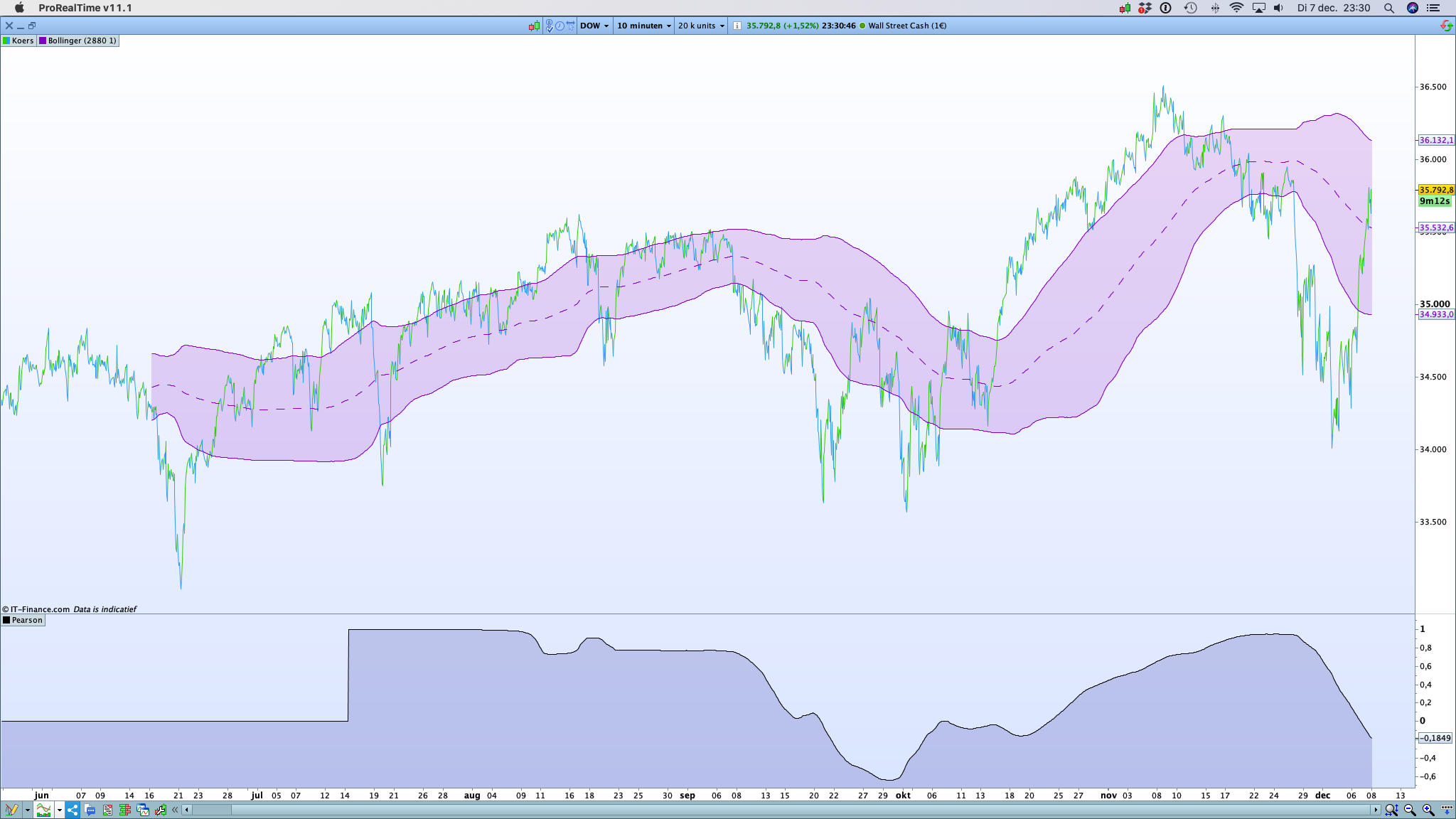
to map the theoretical Gaussian curve to a distribution of "Close" on a defined number of bars.
This allows to have an idea if this distribution (Price) has the contours of a Gaussian curve[attachment file="182879"]

.
See the old version in the indicator library for more information on the other functionalities.

// Quino Statistics Plotter
// By Quino
// version of 05/12/2021
//===================================================================================
// NbrOfSamples : Number of consecutive close
// NbrOfClasses : Number of intervals of values ​​in which we store the values ​​of “close”
// InformationDisplay :
// – false : display of the histogram only
// – true : display of limit values ​​for each class and % of occurrence
// ClassTracer :
// – false : indicator that can be used stand-alone (curve and information)
// – true : indicator usable in the price indicator. By locating the class of the last “close” or another class. Class boundaries are represented by two horizontal lines on the price chart.
// ClassIndex : manual search for the class number corresponding to the last “close” or another class. Alignment of the cue point under the value of the last close (in red)
// GaussianShape
// – false : No Gaussian curve drawn
// – true : Gaussian curve drawn from avrerage and standard deviation of the selected number of consecutive close

//Typical use : NbrOfSamples=150 ; NbrOfClasses=30 (5 samples per class minimum)
//===================================================================================
NbrMaxFrequency=1000 // Number max of occurency per class
AdjustA=30 // Scale calibration
AdjustB=4 // Position calibration
//———————————-
if islastbarupdate then
for k =0 to NbrOfSamples-1 do
$v[k]=close[k]
next
for i= NbrOfSamples-1 downto 0 do
$d[i]=arraymax($v)
for j=NbrOfSamples-1 downto 0 do
if $v[j]=$d[i] then
$v[j]=0
break
endif
next
next
Bin=(arraymax($d)-arraymin($d))/(NbrOfClasses)
For i=0 to NbrOfClasses do
$r[i]=0
next
BinA=arraymin($d)
for j=0 to NbrOfClasses-1 do
Dtemp=0
for i=0 to NbrOfSamples-1 do
if j < NbrOfClasses then
if $d[i]>=BinA+ j*Bin and $d[i] <BinA+(j+1)*Bin then
Dtemp=Dtemp+1
else
if $d[i]>=BinA+ j*Bin and $d[i] =<BinA+(j+1)*Bin then
Dtemp=Dtemp+1
endif
endif
endif
next
$r[j]=Dtemp
next
Vmoy=average[NbrOfSamples](close)
Vect=std[NbrOfSamples](close)
for k =0 to NbrOfClasses-1 do
$Vg[k]=((exp(-0.5*square(((BinA+ k*Bin)-Vmoy)/Vect)))/Vect*sqr(6.18))
next
if GaussianShape Then
Scale=max(arraymax($r),arraymax($Vg))+12
else
Scale=arraymax($r)+12
endif
If scale < AdjustA then
CorrecYY=1
CorrecY=1
endif
For i=1 to (NbrMaxFrequency/AdjustA) do
if scale>=i*AdjustA and scale<(i+1)*AdjustA then
CorrecYY=i+1
CorrecY=(i+1)*AdjustA/AdjustB
endif
next
for i= 0 to NbrOfClasses-1 do
if ClassTracer then
ValCaseMax=(BinA+ClassIndex*Bin)
ValCaseMin=(BinA+(ClassIndex-1)*Bin)
drawsegment(barindex[NbrOfSamples-1-i],ValCaseMax,barindex[NbrOfClasses-i-1],ValCaseMax)coloured (51,153,255)
drawsegment(barindex[NbrOfSamples-1-i],ValCaseMin,barindex[NbrOfClasses-i-1],ValCaseMin)coloured (0,51,153)
if i=ClassIndex then
tag=1
else
tag=undefined
endif
else
drawsegment(barindex[NbrOfClasses-i],$r[i],barindex[NbrOfClasses-i],0)coloured (0,0,0)
drawsegment(barindex[NbrOfClasses-i],$r[i],barindex[NbrOfClasses-i+1],$r[i])coloured (0,0,0)
drawsegment(barindex[NbrOfClasses-i+1],0,barindex[NbrOfClasses-i+1],$r[i]) coloured (0,0,0)
drawpoint(barindex[NbrOfClasses-ClassIndex+1],tag)coloured (0,0,50)
if GaussianShape then
drawsegment(barindex[NbrOfClasses-i+1],$Vg[i],barindex[NbrOfClasses-i],$Vg[i+1])coloured (255,0,0)
endif
if InformationDisplay then
for i= 0 to NbrOfClasses-1 do
temp=round(($r[i]/(NbrOfSamples))*10000)/100
temp1=round((BinA+(i)*Bin),2)
temp2=round((BinA+(i+1)*Bin),2)
drawtext(“%= #temp#”,barindex[NbrOfClasses-i],Scale+CorrecY-2*CorrecYY)coloured (0,0,255)
if close >= temp1 and close < temp2 then
drawtext(“#temp1#”,barindex[NbrOfClasses-i],Scale+CorrecY-6*CorrecYY)coloured (255,0,0)
drawtext(“#temp2#”,barindex[NbrOfClasses-i],Scale+CorrecY-4*CorrecYY)coloured (255,0,0)
else
drawtext(“#temp1#”,barindex[NbrOfClasses-i],Scale+CorrecY-6*CorrecYY)coloured (0,0,0)
drawtext(“#temp2#”,barindex[NbrOfClasses-i],Scale+CorrecY-4*CorrecYY)coloured (0,0,0)
endif
next
drawtext(“Average= #Vmoy#”,barindex-4,Scale-8*CorrecYY)coloured (0,0,0)
drawtext(“STD= #Vect#”,barindex-4,Scale-10*CorrecYY)coloured (0,0,0)
endif
endif
next
endif
if GaussianShape Then
Scale=max(arraymax($r),arraymax($Vg))+12+CorrecY
else
Scale=arraymax($r)+12+CorrecY
endif
if not ClassTracer then
zero=0
else
zero=undefined
Scale=undefined
endif
return Scale as “Vertical Reference”,zero as “Zero”

[attachment file="182879"]

Hello JS,

If you refer to the example of @Bard with the Gaussian curve on the Y axis and compare it with the price curve,
you cannot extract any statistical information.
To calculate a statistic following a Gaussian distribution from the mean and the standard deviation,
you do have to construct the histogram of your series of price "e.g : close" and compare the two shapes of the curves.
If your histogram follows the theoretical Gaussian curve, then you can do a statistical calculation.
If your histogram is different from the theoretical Gaussian curve, then you cannot do this calculation.
(I don't speak about the goodness of fit. It is another history)
The indicator I have created, allows this comparison of curve shapes to be made on any trading supports

Hi JS,
Maybe it’s possible to do it.
It calls a new developement. Not easy to do it.
If I undersand your need, I suggest to use the Bollinger Bands indicator that perform a price analysis from the mean and the SD.
This indicator don’t care if the price curve is a Gausssian distribution or not.
As it is popular in the trading world, il has some interesting properties.

a=(high+low)/2
aa=Average[24](a)
b=STD[10](a)
cl=close

y1=a+1/(b*SQRT(44/7))*exp(-1*(SQUARE((cl[n]-aa)))/2*square(b))
y2=a-1/(b*SQRT(44/7))*exp(-1*(SQUARE((cl[n]-aa)))/2*square(b))

return y1, y2