

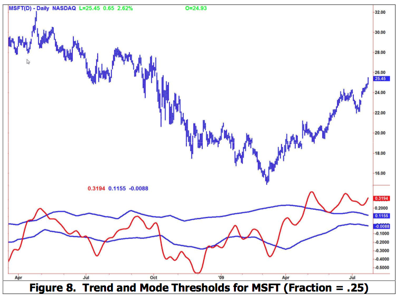
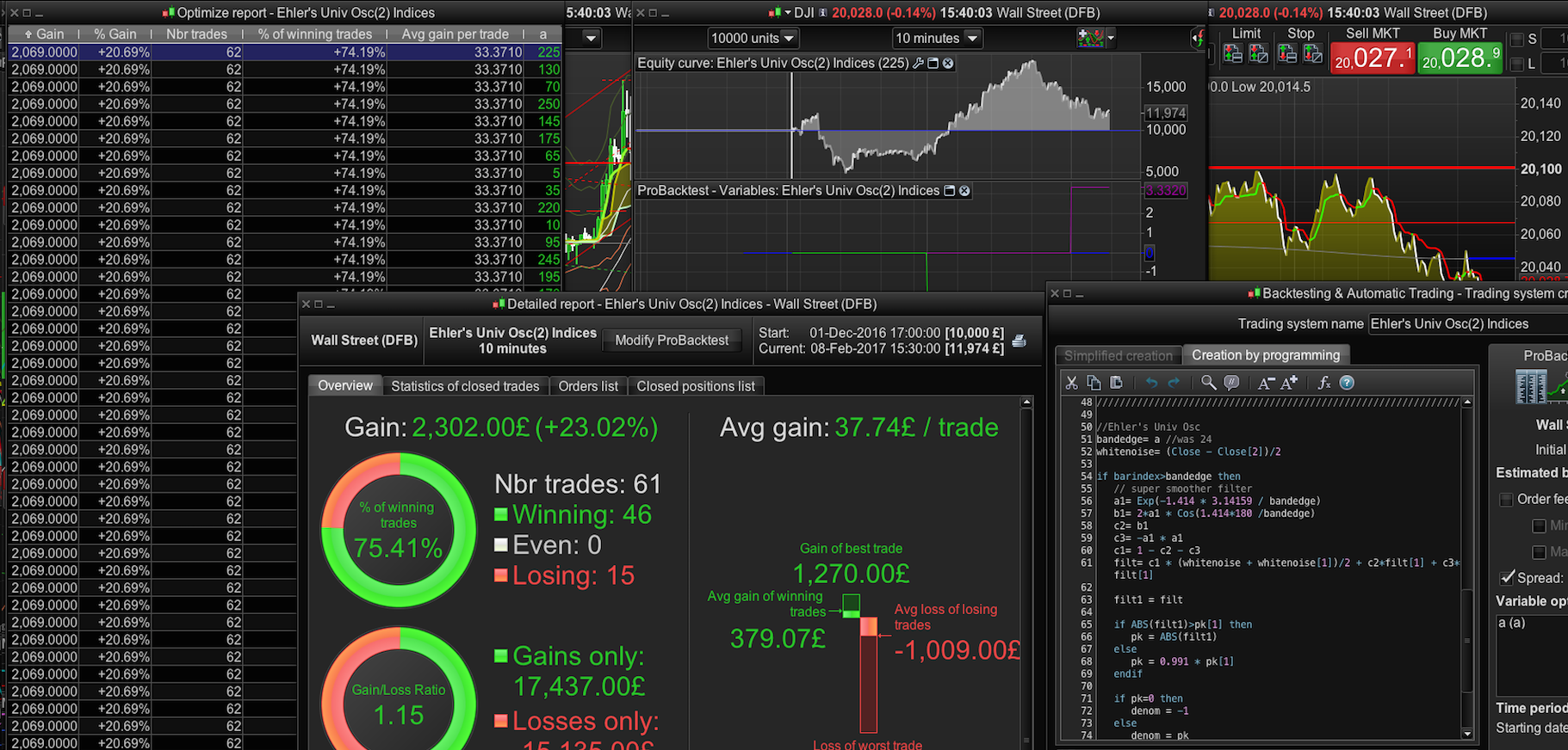
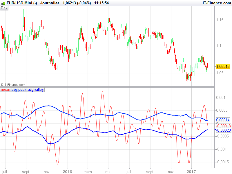
Can anyone code John Ehler's Empirical Mode Decomposition
Viewing 10 posts - 1 through 10 (of 10 total)
Viewing 10 posts - 1 through 10 (of 10 total)
- You must be logged in to reply to this topic.
New Reply
Summary
This topic contains 9 replies,
has 3 voices, and was last updated by ![]()
8 years, 11 months ago.
Topic Details
| Forum: | ProOrder: Automated Strategies & Backtesting |
| Language: | English |
| Started: | 01/24/2017 |
| Status: | Active |
| Attachments: | No files |
Loading...