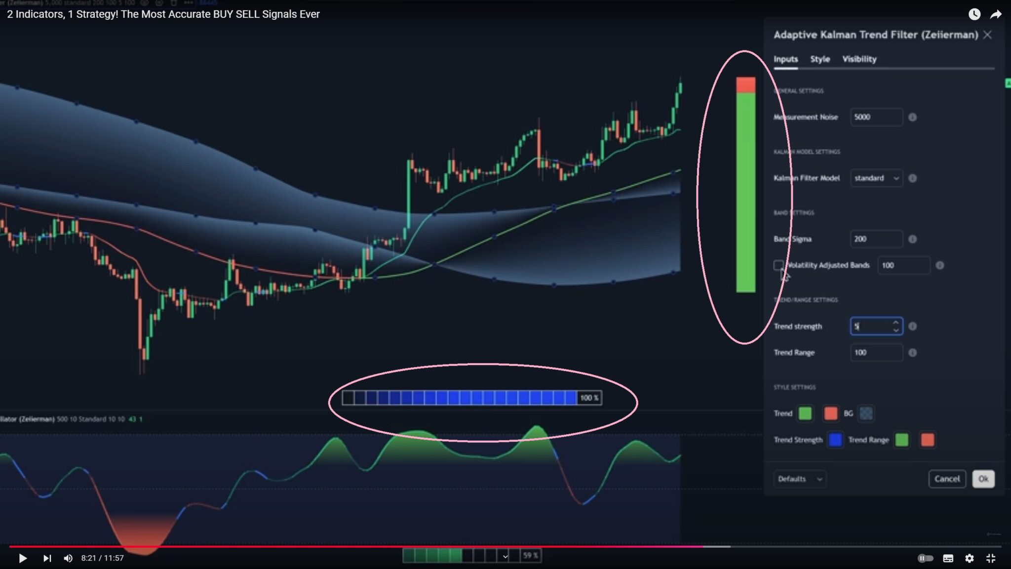
https://youtu.be/_abJdz-UEhM?si=UtRva0cNO2hNoKf0 This indicator offers three distinct Kalman filter models, each designed to handle different market conditions:
Standard Model: This is a conventional Kalman Filter, balancing responsiveness and smoothness. It works well across general market conditions.
Volume-Adjusted Model: In this model, the filter’s measurement noise automatically adjusts based on trading volume. Higher volumes indicate more informative price movements, which the filter treats with higher confidence. Conversely, low-volume movements are treated as less informative, adding robustness during low-activity periods.
Parkinson-Adjusted Model: This model adjusts measurement noise based on price volatility. It uses the price range (high-low) to determine the filter’s sensitivity, making it ideal for handling markets with frequent gaps or spikes. The model responds with higher confidence in low-volatility periods and adapts to high-volatility scenarios by treating them with more caution.
indicator("Adaptive Kalman filter - Trend Strength Oscillator (Zeiierman)", shorttitle = "Kalman Trend Strength Oscillator (Zeiierman)", overlay=false, precision = 0)
//~~}
Adaptive Kalman filter - Trend Strength Oscillator

// This work is licensed under a Attribution-NonCommercial-ShareAlike 4.0 International (CC BY-NC-SA 4.0) https://creativecommons.org/licenses/by-nc-sa/4.0/

// © Zeiierman {
//@version=5
indicator("Adaptive Kalman filter - Trend Strength Oscillator (Zeiierman)", shorttitle = "Kalman Trend Strength Oscillator (Zeiierman)", overlay=false, precision = 0)
//~~}

// ~~ Tooltips {
string t1 = "Process Noise 1: This is the primary noise factor for the Kalman filter process. A higher value increases the filter’s responsiveness to price changes, but may result in less smooth output. Adjust this based on market volatility and the desired balance between smoothness and responsiveness."
string t2 = "Process Noise 2: This is the secondary noise factor for the Kalman filter process. It works in conjunction with Process Noise 1. Increasing this value also makes the filter more responsive but may introduce more noise. Fine-tune this alongside Process Noise 1 for optimal filtering."
string t3 = "Measurement Noise: This value defines the amount of noise in the price data, impacting how much the filter trusts the current price series. Higher values will make the filter rely more on past data, reducing responsiveness. Use this to control the trade-off between smoothness and responsiveness in trending or noisy markets."
string t4 = "Osc Smoothness: Controls the level of smoothing applied to the trend strength oscillator. Higher values result in a smoother oscillator but may cause delays. Lower values make the oscillator more reactive to trend changes, which can be useful for capturing quick reversals or volatility."
string t5 = "Kalman Filter Model: Choose between standard, volume-adjusted, and Parkinson-adjusted Kalman filter models. Volume-adjusted uses trading volume to adapt noise, while Parkinson-adjusted considers price range volatility. Each model impacts how the Kalman filter adjusts to market conditions."
string t6 = "Sigma Lookback: Defines the number of bars used to calculate the standard deviation for confidence bands in the Kalman filter. Higher values use more historical data, which can stabilize the filter in trending markets. Lower values make it more responsive to recent changes."
string t7 = "Trend Lookback: Sets the period over which the trend strength is calculated. Shorter periods make the indicator more sensitive to recent trends, while longer periods smooth the trend, emphasizing longer-term movement."
string t8 = "Strength Smoothness: Defines the level of smoothing applied to the calculated trend strength. Higher values create a more gradual trend strength curve, suitable for identifying persistent trends. Lower values make it more responsive, highlighting shorter-term fluctuations."
//~~~~~~~~~~~~~~~~~~~~~~~~~~~~~~~~~~~~~~~~~~~~~~~~~~~~~~~~~~~~~~~~~~~~~~~~~~~~~~~~~~~~~~~~~~~~~~~~~~~~~~~~~~~~~~~~~~~~~}

// ~~ Parameters {
//@enum     Defines Kalman filter extension models
enum kf_model
    standard = "Standard"
    volume_adjusted = "Volume adjusted"
    parkinson_adjusted = "Parkinson adjusted"
//~~~~~~~~~~~~~~~~~~~~~~~~~~~~~~~~~~~~~~~~~~~~~~~~~~~~~~~~~~~~~~~~~~~~~~~~~~~~~~~~~~~~~~~~~~~~~~~~~~~~~~~~~~~~~~~~~~~~~}

// ~~ Settings {
process_noise_1   = 0.01//input.float(0.01, "Process Noise 1", minval=0.0, maxval=10000, step=0.01, tooltip=t1, group='General settings')
process_noise_2   = 0.01//input.float(0.01, "Process Noise 2", minval=0.0, maxval=10000, step=0.01, tooltip=t2, group='General settings')
measurement_noise = input.float(500.0, "Measurement Noise", minval=0.0, maxval=10000, step=2.0, tooltip=t3, group='General settings')
R1                = input.int(10, title="Osc Smoothness", minval=2, tooltip=t4, group='General settings')
src               = close//input.source(close, "Input Source", tooltip='Primary input to filter', group='General settings')
selected_kf_model = input.enum(kf_model.standard, "Kalman Filter Model", tooltip=t5, group='Kalman Model Settings')
N                 = 500//input.int(500, "Sigma Lookback", minval=2, step=1, tooltip=t6, group='Additional Settings')
N2                = input.int(10, "Trend Lookback", minval=2, step=1, tooltip=t7, group='Trend Settings')
R2                = input.int(10, title="Strength Smoothness", minval=2, tooltip=t8, group='Trend Settings')
pos_col           = input.color(color.lime, title="Trend", inline="style", group='Style Settings')
neu_col           = input.color(color.blue, title="", inline="style", group='Style Settings')
neg_col           = input.color(color.red, title="", inline="style", group='Style Settings')
ob_col            = input.color(color.green, title="OBOS", inline="style1", group='Style Settings')
os_col            = input.color(color.red, title="", inline="style1", group='Style Settings')
bg_col            = input.color(color.rgb(87, 130, 194, 90), title="BG", inline="style2", group='Style Settings')

//~~~~~~~~~~~~~~~~~~~~~~~~~~~~~~~~~~~~~~~~~~~~~~~~~~~~~~~~~~~~~~~~~~~~~~~~~~~~~~~~~~~~~~~~~~~~~~~~~~~~~~~~~~~~~~~~~~~~~}

// ~~ Indicators {
var float filtered_src   = na
var float trend_strength = na
//~~~~~~~~~~~~~~~~~~~~~~~~~~~~~~~~~~~~~~~~~~~~~~~~~~~~~~~~~~~~~~~~~~~~~~~~~~~~~~~~~~~~~~~~~~~~~~~~~~~~~~~~~~~~~~~~~~~~~}

// ~~  Support variables {
var Y_diff     = array.new<float>()
var osc_buffer = array.new<float>()
//~~~~~~~~~~~~~~~~~~~~~~~~~~~~~~~~~~~~~~~~~~~~~~~~~~~~~~~~~~~~~~~~~~~~~~~~~~~~~~~~~~~~~~~~~~~~~~~~~~~~~~~~~~~~~~~~~~~~~}

// ~~  Initialize all KF matrices and vectors {
var F = matrix.new<float>(2, 2, 0.0)
F.set(0, 0, 1.0)
F.set(0, 1, 1.0)
F.set(1, 0, 1.0)

var P = matrix.new<float>(2, 2, 0.0)
matrix.set(P, 0, 0, 1.0)
matrix.set(P, 1, 1, 1.0)

var Q = matrix.new<float>(2, 2, 0.0)
matrix.set(Q, 0, 0, process_noise_1)
matrix.set(Q, 0, 1, process_noise_1 * process_noise_2)
matrix.set(Q, 1, 0, process_noise_2 * process_noise_1)
matrix.set(Q, 1, 1, process_noise_2)

var R = matrix.new<float>(1, 1, measurement_noise)
var H = matrix.new<float>(1, 2, 0.0)
matrix.set(H, 0, 0, 1.0)

var I = matrix.new<float>(2, 2, 0.0)
matrix.set(I, 0, 0, 1.0)
matrix.set(I, 1, 1, 1.0)

var X = array.from(0.0, 0.0)
if barstate.isfirst
    X := array.from(src, src)

if barstate.isconfirmed
    x1 = matrix.get(F, 0, 0) * array.get(X, 0) + matrix.get(F, 0, 1) * array.get(X, 1)
    x2 = matrix.get(F, 1, 1) * array.get(X, 1)
    X := array.from(x1, x2)
    P := F.mult(P.mult(F.transpose())).sum(Q)

    array.push(Y_diff, src - array.get(X, 0))

    R_adjusted = R.copy()
    if selected_kf_model != kf_model.standard and bar_index > 2
        if selected_kf_model == kf_model.volume_adjusted
            matrix.set(R_adjusted, 0, 0, matrix.get(R, 0, 0) * volume[1] / math.min(volume[1], volume))
        else if selected_kf_model == kf_model.parkinson_adjusted
            current_range = high - low
            previous_range = high[1] - low[1]
            range_ratio = current_range / math.max(previous_range, syminfo.mintick)
            parkinson_scaled = 1 + range_ratio
            matrix.set(R_adjusted, 0, 0, matrix.get(R, 0, 0) * parkinson_scaled)

    S = H.mult(P.mult(H.transpose())).sum(R_adjusted)
    K = P.mult(H.transpose().mult(S.inv()))
    innovation = src - array.get(H.mult(X), 0)
    diff = K.mult(innovation)
    X := array.from(array.get(X, 0) + matrix.get(diff, 0, 0), array.get(X, 1) + matrix.get(diff, 1, 0))
    P := I.sum(K.mult(H).mult(-1)).mult(P)

    estimate      = array.get(X, 0)
    oscillator    = array.get(X, 1)
    filtered_src := estimate

    array.push(osc_buffer, oscillator)

    if array.size(Y_diff) >= N
        array.shift(Y_diff)

    if array.size(osc_buffer) >= N2
        A = osc_buffer.abs().max()
        trend_strength := ta.wma((oscillator / A * 100 ),R2)
        array.shift(osc_buffer)
//~~~~~~~~~~~~~~~~~~~~~~~~~~~~~~~~~~~~~~~~~~~~~~~~~~~~~~~~~~~~~~~~~~~~~~~~~~~~~~~~~~~~~~~~~~~~~~~~~~~~~~~~~~~~~~~~~~~~~}

// ~~  Gradient Coloring Logic {
var int num_segments = 10
segment_width        = 100 / num_segments
filled_segments      = math.floor(math.abs(trend_strength) / segment_width)
osc_color            = neu_col

if not na(trend_strength)
    for i = 0 to num_segments - 1
        if i < filled_segments
            osc_color := color.new(trend_strength > 0 ? pos_col : neg_col, 80 - i * 10)
        else
            break
//~~~~~~~~~~~~~~~~~~~~~~~~~~~~~~~~~~~~~~~~~~~~~~~~~~~~~~~~~~~~~~~~~~~~~~~~~~~~~~~~~~~~~~~~~~~~~~~~~~~~~~~~~~~~~~~~~~~~~}

// ~~  Plots {
oscPlot   = plot(ta.wma(trend_strength,R1), color=osc_color, linewidth=3, title="Kalman Trend Strength Oscillator")
kalmanPlot= plot(filtered_src, color=osc_color, linewidth = 2, title="Adaptive Kalman Filter", force_overlay = true)
UpperBand = hline(70, title="70")
midline   = hline(0, title="0")
LowerBand = hline(-70, title="-70")

fill(UpperBand, LowerBand, color=bg_col, title="Background Fill")
midLinePlot = plot(0, color = na, editable = false, display = display.none)
fill(oscPlot, midLinePlot, 80, 30, top_color = color.new(ob_col, 0), bottom_color = color.new(ob_col, 100),  title = "Upper Gradient Fill")
fill(oscPlot, midLinePlot, -30,  -80,  top_color = color.new(os_col, 100), bottom_color = color.new(os_col, 0),  title = "Lower Gradient Fill")
//~~~~~~~~~~~~~~~~~~~~~~~~~~~~~~~~~~~~~~~~~~~~~~~~~~~~~~~~~~~~~~~~~~~~~~~~~~~~~~~~~~~~~~~~~~~~~~~~~~~~~~~~~~~~~~~~~~~~~}

// ~~  Table for Trend Strength {
if barstate.islast
    trend_strength_current = math.round(trend_strength)
    var table trend_table  = table.new(position.bottom_center, num_segments + 1, 1, border_color=chart.fg_color, border_width=1, frame_color=chart.fg_color, frame_width=1)
    for i = 0 to num_segments - 1
        table_segment_color = i < filled_segments ? color.new(trend_strength > 0 ? pos_col : neg_col, 70 - i * 10) : color.new(chart.fg_color, 100)
        table.cell(trend_table, i, 0, "", bgcolor=table_segment_color, width=1, height=2)
    table.cell(trend_table, num_segments, 0, str.tostring(trend_strength_current) + " %", text_color=chart.fg_color, bgcolor=na)
//~~~~~~~~~~~~~~~~~~~~~~~~~~~~~~~~~~~~~~~~~~~~~~~~~~~~~~~~~~~~~~~~~~~~~~~~~~~~~~~~~~~~~~~~~~~~~~~~~~~~~~~~~~~~~~~~~~~~~}
// ~~ Tooltips {
string t1 = “Process Noise 1: This is the primary noise factor for the Kalman filter process. A higher value increases the filter’s responsiveness to price changes, but may result in less smooth output. Adjust this based on market volatility and the desired balance between smoothness and responsiveness.”
string t2 = “Process Noise 2: This is the secondary noise factor for the Kalman filter process. It works in conjunction with Process Noise 1. Increasing this value also makes the filter more responsive but may introduce more noise. Fine-tune this alongside Process Noise 1 for optimal filtering.”
string t3 = “Measurement Noise: This value defines the amount of noise in the price data, impacting how much the filter trusts the current price series. Higher values will make the filter rely more on past data, reducing responsiveness. Use this to control the trade-off between smoothness and responsiveness in trending or noisy markets.”
string t4 = “Osc Smoothness: Controls the level of smoothing applied to the trend strength oscillator. Higher values result in a smoother oscillator but may cause delays. Lower values make the oscillator more reactive to trend changes, which can be useful for capturing quick reversals or volatility.”
string t5 = “Kalman Filter Model: Choose between standard, volume-adjusted, and Parkinson-adjusted Kalman filter models. Volume-adjusted uses trading volume to adapt noise, while Parkinson-adjusted considers price range volatility. Each model impacts how the Kalman filter adjusts to market conditions.”
string t6 = “Sigma Lookback: Defines the number of bars used to calculate the standard deviation for confidence bands in the Kalman filter. Higher values use more historical data, which can stabilize the filter in trending markets. Lower values make it more responsive to recent changes.”
string t7 = “Trend Lookback: Sets the period over which the trend strength is calculated. Shorter periods make the indicator more sensitive to recent trends, while longer periods smooth the trend, emphasizing longer-term movement.”
string t8 = “Strength Smoothness: Defines the level of smoothing applied to the calculated trend strength. Higher values create a more gradual trend strength curve, suitable for identifying persistent trends. Lower values make it more responsive, highlighting shorter-term fluctuations.”
//~~~~~~~~~~~~~~~~~~~~~~~~~~~~~~~~~~~~~~~~~~~~~~~~~~~~~~~~~~~~~~~~~~~~~~~~~~~~~~~~~~~~~~~~~~~~~~~~~~~~~~~~~~~~~~~~~~~~~}
// ~~ Parameters {
//@enum Defines Kalman filter extension models
enum kf_model
standard = “Standard”
volume_adjusted = “Volume adjusted”
parkinson_adjusted = “Parkinson adjusted”
//~~~~~~~~~~~~~~~~~~~~~~~~~~~~~~~~~~~~~~~~~~~~~~~~~~~~~~~~~~~~~~~~~~~~~~~~~~~~~~~~~~~~~~~~~~~~~~~~~~~~~~~~~~~~~~~~~~~~~}
// ~~ Settings {
process_noise_1 = 0.01//input.float(0.01, “Process Noise 1”, minval=0.0, maxval=10000, step=0.01, tooltip=t1, group=’General settings’)
process_noise_2 = 0.01//input.float(0.01, “Process Noise 2”, minval=0.0, maxval=10000, step=0.01, tooltip=t2, group=’General settings’)
measurement_noise = input.float(500.0, “Measurement Noise”, minval=0.0, maxval=10000, step=2.0, tooltip=t3, group=’General settings’)
R1 = input.int(10, title=”Osc Smoothness”, minval=2, tooltip=t4, group=’General settings’)
src = close//input.source(close, “Input Source”, tooltip=’Primary input to filter’, group=’General settings’)
selected_kf_model = input.enum(kf_model.standard, “Kalman Filter Model”, tooltip=t5, group=’Kalman Model Settings’)
N = 500//input.int(500, “Sigma Lookback”, minval=2, step=1, tooltip=t6, group=’Additional Settings’)
N2 = input.int(10, “Trend Lookback”, minval=2, step=1, tooltip=t7, group=’Trend Settings’)
R2 = input.int(10, title=”Strength Smoothness”, minval=2, tooltip=t8, group=’Trend Settings’)
pos_col = input.color(color.lime, title=”Trend”, inline=”style”, group=’Style Settings’)
neu_col = input.color(color.blue, title=””, inline=”style”, group=’Style Settings’)
neg_col = input.color(color.red, title=””, inline=”style”, group=’Style Settings’)
ob_col = input.color(color.green, title=”OBOS”, inline=”style1″, group=’Style Settings’)
os_col = input.color(color.red, title=””, inline=”style1″, group=’Style Settings’)
bg_col = input.color(color.rgb(87, 130, 194, 90), title=”BG”, inline=”style2″, group=’Style Settings’)
//~~~~~~~~~~~~~~~~~~~~~~~~~~~~~~~~~~~~~~~~~~~~~~~~~~~~~~~~~~~~~~~~~~~~~~~~~~~~~~~~~~~~~~~~~~~~~~~~~~~~~~~~~~~~~~~~~~~~~}
// ~~ Indicators {
var float filtered_src = na
var float trend_strength = na
//~~~~~~~~~~~~~~~~~~~~~~~~~~~~~~~~~~~~~~~~~~~~~~~~~~~~~~~~~~~~~~~~~~~~~~~~~~~~~~~~~~~~~~~~~~~~~~~~~~~~~~~~~~~~~~~~~~~~~}
// ~~ Support variables {
var Y_diff = array.new<float>()
var osc_buffer = array.new<float>()
//~~~~~~~~~~~~~~~~~~~~~~~~~~~~~~~~~~~~~~~~~~~~~~~~~~~~~~~~~~~~~~~~~~~~~~~~~~~~~~~~~~~~~~~~~~~~~~~~~~~~~~~~~~~~~~~~~~~~~}
// ~~ Initialize all KF matrices and vectors {
var F = matrix.new<float>(2, 2, 0.0)
F.set(0, 0, 1.0)
F.set(0, 1, 1.0)
F.set(1, 0, 1.0)
var P = matrix.new<float>(2, 2, 0.0)
matrix.set(P, 0, 0, 1.0)
matrix.set(P, 1, 1, 1.0)
var Q = matrix.new<float>(2, 2, 0.0)
matrix.set(Q, 0, 0, process_noise_1)
matrix.set(Q, 0, 1, process_noise_1 * process_noise_2)
matrix.set(Q, 1, 0, process_noise_2 * process_noise_1)
matrix.set(Q, 1, 1, process_noise_2)
var R = matrix.new<float>(1, 1, measurement_noise)
var H = matrix.new<float>(1, 2, 0.0)
matrix.set(H, 0, 0, 1.0)
var I = matrix.new<float>(2, 2, 0.0)
matrix.set(I, 0, 0, 1.0)
matrix.set(I, 1, 1, 1.0)
var X = array.from(0.0, 0.0)
if barstate.isfirst
X := array.from(src, src)
if barstate.isconfirmed
x1 = matrix.get(F, 0, 0) * array.get(X, 0) + matrix.get(F, 0, 1) * array.get(X, 1)
x2 = matrix.get(F, 1, 1) * array.get(X, 1)
X := array.from(x1, x2)
P := F.mult(P.mult(F.transpose())).sum(Q)
array.push(Y_diff, src – array.get(X, 0))
R_adjusted = R.copy()
if selected_kf_model != kf_model.standard and bar_index > 2
if selected_kf_model == kf_model.volume_adjusted
matrix.set(R_adjusted, 0, 0, matrix.get(R, 0, 0) * volume[1] / math.min(volume[1], volume))
else if selected_kf_model == kf_model.parkinson_adjusted
current_range = high – low
previous_range = high[1] – low[1]
range_ratio = current_range / math.max(previous_range, syminfo.mintick)
parkinson_scaled = 1 + range_ratio
matrix.set(R_adjusted, 0, 0, matrix.get(R, 0, 0) * parkinson_scaled)
S = H.mult(P.mult(H.transpose())).sum(R_adjusted)
K = P.mult(H.transpose().mult(S.inv()))
innovation = src – array.get(H.mult(X), 0)
diff = K.mult(innovation)
X := array.from(array.get(X, 0) + matrix.get(diff, 0, 0), array.get(X, 1) + matrix.get(diff, 1, 0))
P := I.sum(K.mult(H).mult(-1)).mult(P)
estimate = array.get(X, 0)
oscillator = array.get(X, 1)
filtered_src := estimate
array.push(osc_buffer, oscillator)
if array.size(Y_diff) >= N
array.shift(Y_diff)
if array.size(osc_buffer) >= N2
A = osc_buffer.abs().max()
trend_strength := ta.wma((oscillator / A * 100 ),R2)
array.shift(osc_buffer)
//~~~~~~~~~~~~~~~~~~~~~~~~~~~~~~~~~~~~~~~~~~~~~~~~~~~~~~~~~~~~~~~~~~~~~~~~~~~~~~~~~~~~~~~~~~~~~~~~~~~~~~~~~~~~~~~~~~~~~}
// ~~ Gradient Coloring Logic {
var int num_segments = 10
segment_width = 100 / num_segments
filled_segments = math.floor(math.abs(trend_strength) / segment_width)
osc_color = neu_col
if not na(trend_strength)
for i = 0 to num_segments – 1
if i < filled_segments
osc_color := color.new(trend_strength > 0 ? pos_col : neg_col, 80 – i * 10)
else
break
//~~~~~~~~~~~~~~~~~~~~~~~~~~~~~~~~~~~~~~~~~~~~~~~~~~~~~~~~~~~~~~~~~~~~~~~~~~~~~~~~~~~~~~~~~~~~~~~~~~~~~~~~~~~~~~~~~~~~~}
// ~~ Plots {
oscPlot = plot(ta.wma(trend_strength,R1), color=osc_color, linewidth=3, title=”Kalman Trend Strength Oscillator”)
kalmanPlot= plot(filtered_src, color=osc_color, linewidth = 2, title=”Adaptive Kalman Filter”, force_overlay = true)
UpperBand = hline(70, title=”70″)
midline = hline(0, title=”0″)
LowerBand = hline(-70, title=”-70″)
fill(UpperBand, LowerBand, color=bg_col, title=”Background Fill”)
midLinePlot = plot(0, color = na, editable = false, display = display.none)
fill(oscPlot, midLinePlot, 80, 30, top_color = color.new(ob_col, 0), bottom_color = color.new(ob_col, 100), title = “Upper Gradient Fill”)
fill(oscPlot, midLinePlot, -30, -80, top_color = color.new(os_col, 100), bottom_color = color.new(os_col, 0), title = “Lower Gradient Fill”)
//~~~~~~~~~~~~~~~~~~~~~~~~~~~~~~~~~~~~~~~~~~~~~~~~~~~~~~~~~~~~~~~~~~~~~~~~~~~~~~~~~~~~~~~~~~~~~~~~~~~~~~~~~~~~~~~~~~~~~}
// ~~ Table for Trend Strength {
if barstate.islast
trend_strength_current = math.round(trend_strength)
var table trend_table = table.new(position.bottom_center, num_segments + 1, 1, border_color=chart.fg_color, border_width=1, frame_color=chart.fg_color, frame_width=1)
for i = 0 to num_segments – 1
table_segment_color = i < filled_segments ? color.new(trend_strength > 0 ? pos_col : neg_col, 70 – i * 10) : color.new(chart.fg_color, 100)
table.cell(trend_table, i, 0, “”, bgcolor=table_segment_color, width=1, height=2)
table.cell(trend_table, num_segments, 0, str.tostring(trend_strength_current) + ” %”, text_color=chart.fg_color, bgcolor=na)
//~~~~~~~~~~~~~~~~~~~~~~~~~~~~~~~~~~~~~~~~~~~~~~~~~~~~~~~~~~~~~~~~~~~~~~~~~~~~~~~~~~~~~~~~~~~~~~~~~~~~~~~~~~~~~~~~~~~~~}
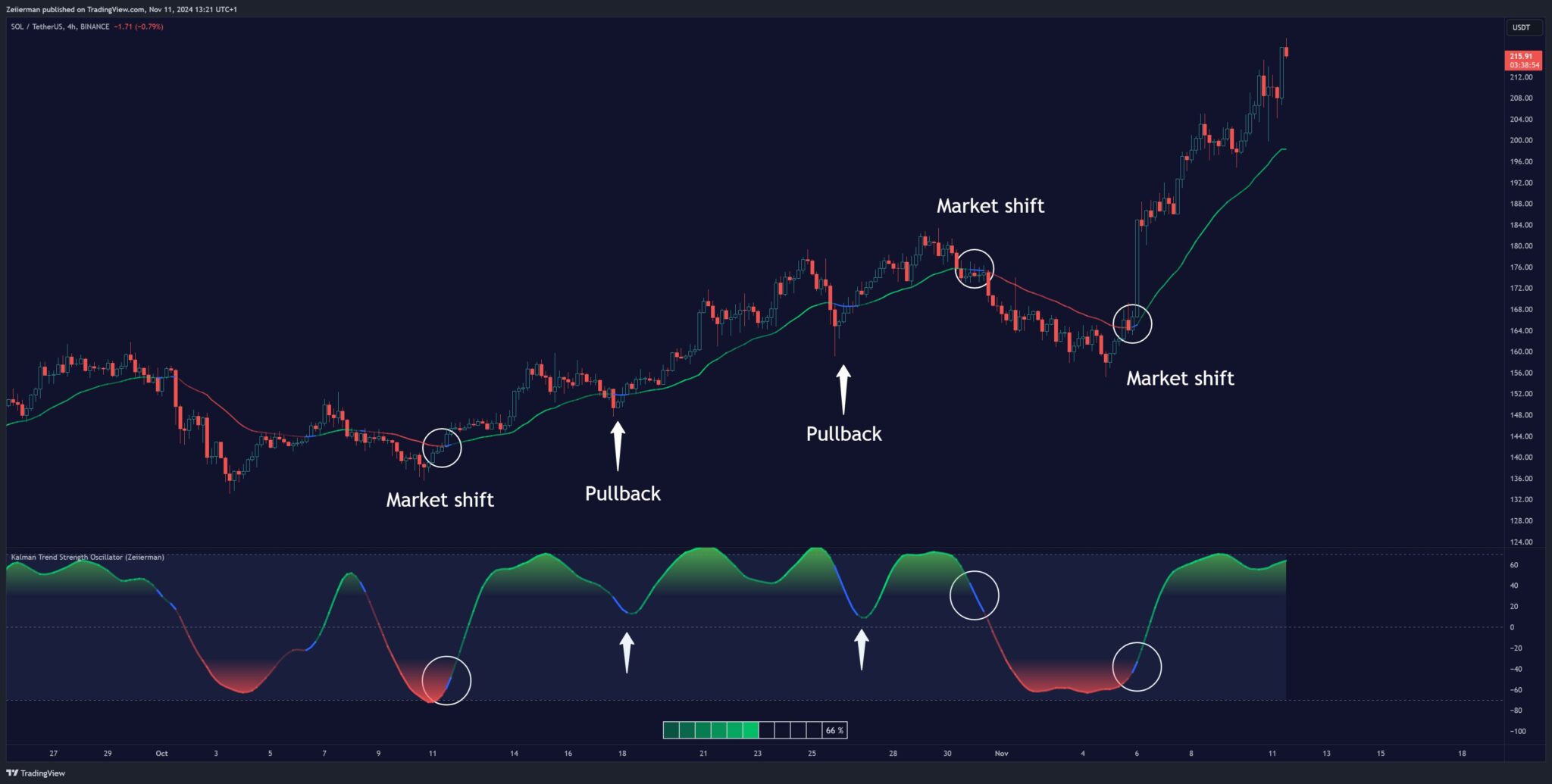
The Adaptive Kalman Filter – Trend Strength Oscillator by Zeiierman is a sophisticated trend-following indicator that uses advanced mathematical techniques, including vector and matrix operations, to decompose price movements into trend and oscillatory components. Unlike standard indicators, this model assumes that price is driven by two latent (unobservable) factors: a long-term trend and localized oscillations around that trend. Through a dynamic “predict and update” process, the Kalman Filter leverages vectors to adaptively separate these components, extracting a clearer view of market direction and strength.