Introduction

Every linear regression channel on a chart shares one hidden assumption: that all the bars in the window deserve the same say in where the line goes. Sixty closes go in, one straight line comes out, and the bar printed in the middle of a violent gap-and-reverse session counts exactly as much as the bar printed in a quiet, orderly drift.

That assumption is convenient and it is also wrong. Volatility clusters. A sixty bar window almost never contains sixty bars of the same quality: it contains a calm stretch and a chaotic one, and the chaotic stretch drags the line around far more than it should.

The Variance-Weighted Regression Trend, designed by BackQuant, fixes that by letting each bar vote with a weight inversely proportional to its own local variance. Quiet stretches drive the line. Noisy stretches are pushed aside. Everything else the indicator draws — the channel, the trend state, the forward projection — is read off that weighted fit, and the fit reports its own quality so you can see when it deserves to be believed.

Theory Behind the Indicator

The calculation runs in four stages.

Stage one: a plain fit, to find out who is behaving badly. An ordinary least squares line is fitted through the last regLen bars and the residual of every bar is measured — how far that bar closed from the line. Squaring those residuals gives each bar an error energy.

Stage two: turn the residuals into a local variance. The squared residuals are smoothed forward through the window, from the oldest bar to the newest, with an exponential average, a Wilder average or a simple rolling mean. The result is a variance estimate that belongs to a region of the window rather than to a single bar: a run of wild bars raises the variance for the whole run, one isolated bar barely moves it.

A regularisation term is added on top. A fixed fraction of the mean residual variance of the window goes into every local estimate, so that a bar which happens to land exactly on the line cannot claim a variance of zero and therefore an infinite weight. This is the single parameter that keeps the whole scheme stable, and it is worth understanding before touching it.

Stage three: from variance to weight. Each bar gets a raw weight of

weight = 1 / variance ^ power

with power = 0 giving every bar the same weight — an ordinary regression — power = 1 giving true inverse variance weighting, and higher values punishing noisy bars far more aggressively. Raw weights are then divided by the average raw weight of the window, which makes them relative and scale free, and clipped into a [minimum, maximum] band so that no single bar can dominate and no bar can be silenced completely.

Stage four: the weighted fit. The line is refitted with those weights. From the weighted moments the indicator also derives, at no extra cost, four numbers that describe how good the fit actually is:

• the weighted R², the share of the weighted variation the line explains
• the weighted residual RMS, the typical distance from price to line once weights are applied — this is what sets the channel width by default
• the regression standard error, the uncertainty of the fitted value at the current bar, the alternative channel base
• the effective sample size, (Σw)² / Σw², which answers the interesting question: out of sixty bars, how many are really deciding this line?

That last one is the number worth watching. In a window of homogeneous noise the weights come out nearly equal and the effective sample size sits close to the window length. In a window that straddles a volatility regime change it collapses. On a synthetic series alternating eighty quiet bars with eighty noisy ones, a sixty bar window shows a median effective sample size of about 41 bars and drops as low as 15 — meaning that in the worst stretches a quarter of the window is doing all the work and the rest is switched off.

Where the Weighting Actually Changes Something

It is worth being precise about this, because it sets expectations.

Measuring the distance between the weighted line and a plain unweighted one, in units of the residual RMS, on synthetic series of 60 bar windows:

• on a series with alternating volatility regimes: median 0.30, 90th percentile 1.23, up to 2.24
• on a homogeneous trending series: median 0.15
• on a homogeneous ranging series: median 0.16

In other words, the mechanism only separates from an ordinary regression when the window is genuinely heterogeneous. When every bar in the window carries the same amount of noise, the weights come out flat and you get an ordinary regression back. That is the correct behaviour: it does not manufacture a difference where there is nothing to correct. Just do not expect it to look dramatically different on a calm instrument in a calm session.

The Trend State and Its Quality Gate

The trend is the sign of the weighted slope: up while it is positive, down while it is negative, and it holds its last state rather than flickering around zero.

On top of that sits an optional quality gate. When it is on, a flip is only accepted if the weighted R² clears a minimum and the ratio of slope to slope standard error clears another. The intent is to stop the line from flipping on a slope that is statistically indistinguishable from flat.

It does reduce flips — on synthetic series, from 29 to 15 in a range and from 13 to 7 in a trend — but it is honest to say what it is and what it is not. The slope standard error is the classical least squares formula, and that formula assumes independent residuals. Residuals of a line fitted to prices are strongly autocorrelated: measured on the same synthetic series, the lag one autocorrelation of the weighted residuals runs around +0.83. At that level the classical standard error understates the true uncertainty by roughly a factor of three. A slope score of 8 is therefore not a t statistic of 8; read as one, it is closer to 2.5.

The practical consequence: the default minSlopeScore of 0.50 is essentially never binding, and if you want that threshold to mean something statistical you should be setting it three or four times higher. The R² threshold does more of the work. Treat the gate as a smoothing device with a sensible shape rather than as a significance test, and it earns its place.

Key Features at a Glance

• Least squares fit weighted by each bar’s own local variance, so volatile stretches lose influence over the line
• Three variance models: exponential, Wilder and rolling mean
• Weight aggressiveness from flat (an ordinary regression) through true inverse variance to heavily punitive
• Regularisation and weight clipping, so no bar can take over the fit and none is fully silenced
• Channel width from either the weighted residual RMS or the regression standard error
• Optional channel expansion while the fit is poor, so the envelope widens exactly when the line deserves less trust
• Trend state with an optional quality gate on weighted R² and slope score
• Forward projection track from the fitted slope
• Halo around the line that breathes with trend strength, plus a short bloom on every flip
• Candles repainted with the trend colour

How to Read the Indicator

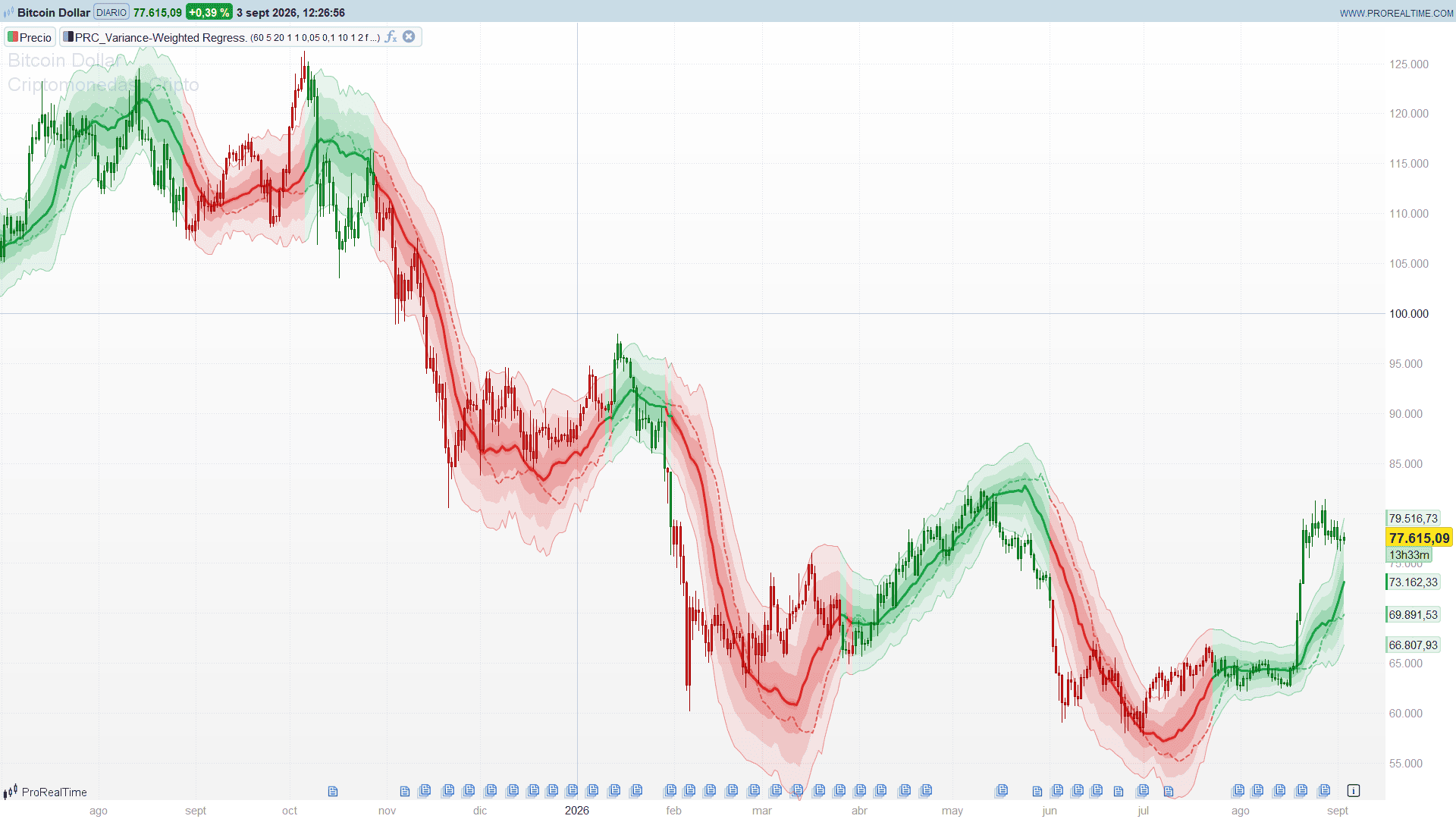
The thick central line is the weighted fit. Its colour is the trend state: green while the weighted slope is positive, red while it is negative.

The two thin rails are the channel. With the default base — weighted residual RMS — the rails sit at a multiple of the typical weighted distance from price to line, which makes them a conditional volatility envelope: they narrow when the bars that matter are behaving and widen when they are not. Switching the base to the regression standard error changes the meaning entirely: the rails then measure the uncertainty of the line itself, not the dispersion of price around it, and they come out much tighter.

The shading between line and rails fades outwards in three steps, so the eye reads the zone immediately around the line as the high confidence area.

The halo around the line is trend strength: a blend of weighted R² and slope score, capped. A thick, solid halo means the line explains the window well and the slope is steep relative to its own uncertainty. A thin, faint halo means the fit is loose and the direction is soft. When the state flips, the halo blooms for three bars and then settles.

The dotted line is the projection track. It shows, at each bar, where the fit issued a few bars earlier said price would be by now — a running record of the forecast against what the market actually did. When it hugs price, the slope has been a good extrapolation; when it drifts away repeatedly, the window is fitting a direction the market is not following.

Practical Applications

As a trend filter with a built in confidence reading. The pairing that matters is direction plus effective sample size. A green line whose halo is thick and whose window is homogeneous is a different object from a green line held up by a handful of quiet bars in an otherwise chaotic window. The first is a trend; the second is an artefact of the weighting, and it will flip.

As an adaptive channel. With the residual RMS base, the rails give a mean reversion envelope that already discounts the bars that were misbehaving. Touches of the outer rail while the halo is thick tend to be stretches within a trend; touches while the halo is thin are more often just noise in a window with no direction.

As a regime detector. Turn on the poor fit expansion. The channel then widens precisely when weighted R² falls, which is a visual way of saying “this window has no line in it”. A channel that has been breathing outwards for twenty bars is telling you the linear model has stopped describing this market, regardless of what colour the line is.

On the variance model. The exponential default reacts fastest to a change in noise regime. Wilder is slower and steadier, and gives a line that flips less. The rolling mean is the bluntest of the three, with a hard window: a violent bar is fully weighted until it leaves the variance window, then vanishes at once. Choose by how quickly you want the indicator to forgive a shock.

Indicator Configuration

Price source is taken from the platform’s own source selector in the indicator settings.

• regLen (default: 60): regression window in bars, from 10 to 300
• projBars (default: 5): how many bars ahead the fitted line is extended
• varLen (default: 20): smoothing length of the local variance, from 2 to 100
• varMode (default: 1): variance model. 1 = exponential, 2 = Wilder, 3 = rolling mean
• wPower (default: 1.0): weight aggressiveness. 0 = equal weights, 1 = inverse variance, above 1 suppresses high variance bars harder
• varReg (default: 0.05): regularisation. Fraction of the mean residual variance added to every local estimate. Lower it towards 0 for a sharper, twitchier fit; raise it towards 0.3 for a fit that behaves like an ordinary regression
• minW (default: 0.10): floor for the relative weight of a bar
• maxW (default: 10.0): ceiling for the relative weight of a bar
• chanMode (default: 1): channel base. 1 = weighted residual RMS, 2 = regression standard error
• chanMult (default: 2.0): channel half width in units of that base
• expandBad (default: 0): set to 1 to widen the channel while the fit is poor
• badExpand (default: 0.50): how much wider it gets at R² = 0
• qualGate (default: 0): set to 1 to require a minimum fit quality before a flip is accepted
• minR2v (default: 0.15): minimum weighted R² required to flip
• minScore (default: 0.50): minimum slope over standard error required to flip
• showChan (default: 1): draw the channel rails
• showFill (default: 1): shade the channel
• showGlow (default: 1): draw the halo and the flip bloom
• showProj (default: 1): plot the projection track
• showOLS (default: 0): plot the plain unweighted fit for comparison
• paintBar (default: 1): repaint the candles with the trend colour
• bullR / bullG / bullB, bearR / bearG / bearB, olsR / olsG / olsB: colours

Two Settings Worth Experimenting With

Set wPower to 0 and turn on showOLS. With flat weights the indicator becomes an ordinary regression, and the reference line should sit exactly underneath it. That is the cleanest way to see how much work the weighting is doing on your instrument: raise wPower back up and watch the two lines separate. If they never separate much, your window is homogeneous and you can save yourself the computation.

Lower varLen well below regLen. With varLen at 5 and regLen at 60, the variance estimate becomes very local and the weighting turns into something close to a shock filter: a single turbulent cluster is nearly excised from the fit. With varLen close to regLen the variance is almost constant across the window and the weighting flattens out. This ratio, more than wPower, controls the character of the indicator.

The Code

//----------------------------------------------
//PRC_Variance-Weighted Regression Trend
//version = 1
//03.09.2026
//Ivan Gonzalez @ www.prorealcode.com
//Concept and design: BackQuant - Mozilla Public License 2.0
//Sharing ProRealTime knowledge
//----------------------------------------------
// Overlay indicator. A least squares fit in which each bar of the window votes
// with a weight inversely proportional to its OWN local variance: the quiet
// stretches drive the line and the noisy ones are pushed aside. The channel, the
// trend state and the projection are all read off that weighted fit, and the fit
// reports its own quality (weighted R2 and slope over standard error) so a trend
// flip can be required to clear a statistical bar before it is accepted.
//----------------------------------------------


// === 1. REGRESSION ===
// Price source is the one selected in the indicator settings panel (customclose).
regLen   = 60      // regression window in bars, 10 to 300
projBars = 5       // bars the fitted line is extended forward, 1 to 50


// === 2. VARIANCE WEIGHTING ===
varLen   = 20      // smoothing length of the local variance, 2 to 100
varMode  = 1       // 1 = EMA, 2 = RMA (Wilder), 3 = rolling mean
wPower   = 1.0     // 0 = equal weights, 1 = inverse variance, above 1 = harsher
varReg   = 0.05    // regularisation: fraction of the mean residual variance added
                   // to every local estimate, so a near zero variance cannot take
                   // over the whole fit
minW     = 0.10    // floor for the relative weight of a bar
maxW     = 10.0    // ceiling for the relative weight of a bar


// === 3. CHANNEL ===
chanMode  = 1      // 1 = weighted residual RMS, 2 = regression standard error
chanMult  = 2.0    // channel half width, in units of the base chosen above
expandBad = 0      // 1 = widen the channel while the fit is poor
badExpand = 0.50   // how much wider it gets at R2 = 0


// === 4. TREND ===
qualGate = 0       // 1 = a flip needs a minimum fit quality to be accepted
minR2v   = 0.15    // minimum weighted R2 required to flip
minScore = 0.50    // minimum |slope| / slope standard error required to flip


// === 5. DISPLAY ===
showChan = 1       // 1 = draw the channel rails
showFill = 1       // 1 = shade the channel (three steps, fading outwards)
showGlow = 1       // 1 = halo around the line, wider the stronger the trend
showProj = 1       // 1 = plot the projection track (see note below)
showOLS  = 0       // 1 = plot the plain unweighted least squares line for comparison
paintBar = 1       // 1 = repaint the candles with the trend colour
                   // line thickness is the literal 3 in the RETURN at the end of
                   // the code: STYLE() only takes a literal, never a variable
bullR = 22         // bullish colour. Medium tones on purpose: the default chart
bullG = 163        // background in ProRealTime is white, and a pure #00FF00 has a
bullB = 74         // contrast ratio of 1.37 to 1 against it, which is invisible
bearR = 220        // bearish colour
bearG = 38
bearB = 38
olsR = 113         // unweighted least squares reference line
olsG = 128
olsB = 150


//----------------------------------------------
// WARM UP COUNTER
// nCalc counts CALCULATED bars, not chart bars, so the guard still holds if the
// optional DEFPARAM CALCULATEONLASTBARS at the bottom of this header is enabled.
//----------------------------------------------
once nCalc = 0
once trendSt = 0
nCalc = nCalc + 1


if nCalc > regLen + 3 then
   ready = 1
else
   ready = 0
endif


trQual = 0
chanW = 0
wgtR2 = 0
slpScore = 0


if ready = 1 then


   //----------------------------------------------
   // 1. THE UNWEIGHTED FIT AND ITS RESIDUAL ENERGY, IN CLOSED FORM
   //
   // LinearRegression[n] is the value of the least squares line ON the current
   // bar, so with the plain mean it also gives the slope:
   //       fit(current) = mean + slope * (n - 1) / 2
   // and the total residual energy of that fit needs no loop either:
   //       SSE = Syy - slope^2 * Sxx     with Sxx = n(n^2-1)/12 for x = 0..n-1
   // That identity removes one full pass over the window: the naive form walks
   // the window once more just to add the squared residuals up.
   //----------------------------------------------
   olsVal = LinearRegression[regLen](customclose)
   meanY  = average[regLen](customclose)
   olsSlp = 2 * (olsVal - meanY) / (regLen - 1)


   syy  = summation[regLen](customclose * customclose) - regLen * meanY * meanY
   sxxC = regLen * (regLen * regLen - 1) / 12
   resSum = max(0, syy - olsSlp * olsSlp * sxxC)


   meanRes2 = resSum / regLen
   varFloor = max(meanRes2 * varReg, pointsize * pointsize)


   //----------------------------------------------
   // 2. LOCAL VARIANCE AND RAW WEIGHTS, IN ONE PASS
   // The variance is smoothed forward through the window, from the oldest bar to
   // the newest, which is what makes it local to a region of the window instead of
   // global. Because the floor above is already known, the raw weight of each bar
   // can be built in the same pass.
   //----------------------------------------------
   if varMode = 1 then
      alphaV = 2 / (varLen + 1)
   elsif varMode = 2 then
      alphaV = 1 / varLen
   else
      alphaV = 0
   endif


   rawSum = 0
   vState = 0
   rollSum = 0
   seeded = 0


   for j = 0 to regLen - 1 do
      i = regLen - 1 - j
      fitted = olsVal - olsSlp * i
      resid = customclose[i] - fitted
      res2 = resid * resid
      $sqRes[i] = res2


      if varMode = 3 then
         rollSum = rollSum + res2
         if j >= varLen then
            oldIdx = regLen - 1 - j + varLen
            rollSum = rollSum - $sqRes[oldIdx]
         endif
         vState = rollSum / min(j + 1, varLen)
      elsif seeded = 0 then
         vState = res2
         seeded = 1
      else
         vState = alphaV * res2 + (1 - alphaV) * vState
      endif


      vLoc = max(vState + varFloor, 0.000000000001)


      if wPower = 0 then
         raww = 1
      elsif wPower = 1 then
         raww = 1 / vLoc
      else
         raww = exp(0 - wPower * log(vLoc))
      endif


      $rawW[i] = raww
      rawSum = rawSum + raww
   next


   avgRaw = rawSum / regLen


   //----------------------------------------------
   // 3. WEIGHTED MOMENTS
   // swyy, the weighted sum of y squared, is the extra moment that lets the
   // weighted SSE and SST be written in closed form below, which removes a third
   // pass over the window.
   //----------------------------------------------
   sw = 0
   sw2 = 0
   swx = 0
   swy = 0
   swxx = 0
   swxy = 0
   swyy = 0


   for i = 0 to regLen - 1 do
      xVal = regLen - 1 - i
      yVal = customclose[i]
      wVal = max(minW, min(maxW, $rawW[i] / avgRaw))
      sw = sw + wVal
      sw2 = sw2 + wVal * wVal
      swx = swx + wVal * xVal
      swy = swy + wVal * yVal
      swxx = swxx + wVal * xVal * xVal
      swxy = swxy + wVal * xVal * yVal
      swyy = swyy + wVal * yVal * yVal
   next


   //----------------------------------------------
   // 4. THE WEIGHTED LINE
   //----------------------------------------------
   wDen = sw * swxx - swx * swx
   if wDen <> 0 then
      wSlope = (sw * swxy - swx * swy) / wDen
   else
      wSlope = 0
   endif
   wInter = (swy - wSlope * swx) / sw
   regVal = wInter + wSlope * (regLen - 1)
   projVal = regVal + wSlope * projBars


   //----------------------------------------------
   // 5. QUALITY OF THE FIT
   //     SSE = swyy + a^2*sw + b^2*swxx - 2a*swy - 2b*swxy + 2ab*swx
   //     SST = swyy - swy^2 / sw
   // Both are exact expansions of the sums a third pass would accumulate one bar
   // at a time. max(0, ...) is there because the expansion of a difference of
   // squares can land on a small negative in floating point, and sqrt of that
   // would poison everything downstream.
   //----------------------------------------------
   sse = swyy + wInter * wInter * sw + wSlope * wSlope * swxx
   sse = sse - 2 * wInter * swy - 2 * wSlope * swxy + 2 * wInter * wSlope * swx
   sse = max(0, sse)
   sst = max(0, swyy - swy * swy / sw)


   resRms = sqrt(sse / sw)


   if sst > 0 then
      wgtR2 = max(0, min(1, 1 - sse / sst))
   else
      wgtR2 = 0
   endif


   resVar = sse / (regLen - 2)
   xMean = swx / sw
   cSxx = swxx - swx * swx / sw


   slpScore = 0
   regSE = 0
   if cSxx > 0 then
      slpVar = resVar / cSxx
      if slpVar > 0 then
         slpScore = abs(wSlope) / sqrt(slpVar)
      endif
      fitVar = resVar * (1 / sw + (regLen - 1 - xMean) * (regLen - 1 - xMean) / cSxx)
      if fitVar > 0 then
         regSE = sqrt(fitVar)
      endif
   endif


   //----------------------------------------------
   // 6. TREND STATE
   //----------------------------------------------
   qPass = 1
   if qualGate = 1 then
      qPass = 0
      if wgtR2 >= minR2v and slpScore >= minScore then
         qPass = 1
      endif
   endif


   if trendSt = 0 then
      if wSlope >= 0 then
         trendSt = 1
      else
         trendSt = 2
      endif
   elsif wSlope > 0 and trendSt <> 1 and qPass = 1 then
      trendSt = 1
   elsif wSlope < 0 and trendSt <> 2 and qPass = 1 then
      trendSt = 2
   endif


   //----------------------------------------------
   // 7. CHANNEL
   //----------------------------------------------
   if chanMode = 1 then
      chanBase = resRms
   else
      chanBase = regSE
   endif


   fitExp = 1
   if expandBad = 1 then
      fitExp = 1 + (1 - wgtR2) * badExpand
   endif


   chanW = chanBase * chanMult * fitExp


   //----------------------------------------------
   // 8. TREND STRENGTH, USED BY THE HALO
   //----------------------------------------------
   trQual = min(max(0, min(wgtR2, 1)) * 0.60 + max(0, min(slpScore / 3, 1)) * 0.40, 1)


endif


//----------------------------------------------
// FLIPS AND THE BLOOM THAT FOLLOWS THEM
// The bloom is driven by the bar count since the last flip, which is 0 on the flip
// bar itself and only then starts the fade, so the halo swells one bar AFTER the
// turn rather than on it. That is deliberate.
//----------------------------------------------
flipNow = 0
if trendSt = 1 and trendSt[1] = 2 then
   flipNow = 1
endif
if trendSt = 2 and trendSt[1] = 1 then
   flipNow = 1
endif


bloomS = 0
if flipNow[1] = 1 then
   bloomS = 1.00
elsif flipNow[2] = 1 then
   bloomS = 0.55
elsif flipNow[3] = 1 then
   bloomS = 0.25
endif


//----------------------------------------------
// COLOUR
//----------------------------------------------
if trendSt = 1 then
   cR = bullR
   cG = bullG
   cB = bullB
elsif trendSt = 2 then
   cR = bearR
   cG = bearG
   cB = bearB
else
   cR = 113
   cG = 128
   cB = 150
endif


//----------------------------------------------
// CHANNEL RAILS AND THE THREE STEP SHADING
// A gradient fill is not available, so the half channel is split into three bands
// with decreasing alpha. fScale collapses all six series onto the regression line
// when the shading is off: a fill of zero area, which is the safe way to switch a
// COLORBETWEEN off (calling it inside a per bar IF is not).
//----------------------------------------------
if showChan = 1 then
   upLine = regVal + chanW
   dnLine = regVal - chanW
else
   upLine = undefined
   dnLine = undefined
endif


fScale = 0
if showChan = 1 and showFill = 1 then
   fScale = 1
endif


fu1 = regVal + chanW * fScale / 3
fu2 = regVal + chanW * fScale * 2 / 3
fu3 = regVal + chanW * fScale
fl1 = regVal - chanW * fScale / 3
fl2 = regVal - chanW * fScale * 2 / 3
fl3 = regVal - chanW * fScale


colorbetween(regVal, fu1, cR, cG, cB, 100)
colorbetween(fu1, fu2, cR, cG, cB, 55)
colorbetween(fu2, fu3, cR, cG, cB, 24)
colorbetween(regVal, fl1, cR, cG, cB, 100)
colorbetween(fl1, fl2, cR, cG, cB, 55)
colorbetween(fl2, fl3, cR, cG, cB, 24)


//----------------------------------------------
// HALO
// Two bands whose width breathes with the trend strength, plus a third that
// swells for three bars after a flip. Same zero area trick to switch them off.
//----------------------------------------------
gScale = 0
if showGlow = 1 then
   gScale = 1
endif


atrV = averagetruerange[14](close)
glowW = atrV * (0.035 + trQual * 0.030) * gScale
outerW = glowW * 2.4


bloomW = 0
if bloomS > 0 then
   bloomW = atrV * (0.10 + bloomS * 0.10) * gScale
endif


aOuter = round(255 * (5 + trQual * 8) / 100)
aInner = round(255 * (14 + trQual * 22) / 100)
aBloom = round(255 * (10 + bloomS * 18) / 100)


outLo = regVal - outerW
outHi = regVal + outerW
inLo = regVal - glowW
inHi = regVal + glowW
blLo = regVal - bloomW
blHi = regVal + bloomW


colorbetween(outLo, outHi, cR, cG, cB, aOuter)
colorbetween(inLo, inHi, cR, cG, cB, aInner)
colorbetween(blLo, blHi, cR, cG, cB, aBloom)


//----------------------------------------------
// PROJECTION
// A returned series stops at the current bar, so the projection is drawn where it
// does exist: at bar t the value plotted is the projection issued
// projBars bars ago. It is the whole forward track minus the last projBars bars,
// and it reads as a running record of the forecast against what price actually
// did.
//----------------------------------------------
if showProj = 1 then
   projLine = projVal[projBars]
else
   projLine = undefined
endif


if showOLS = 1 then
   olsLine = olsVal
else
   olsLine = undefined
endif


//----------------------------------------------
// TREND CANDLES
//----------------------------------------------
if paintBar = 1 and ready = 1 then
   drawcandle(open, high, low, close) coloured(cR, cG, cB)
endif


RETURN regVal COLOURED(cR, cG, cB) STYLE(line, 3) AS "VW Regression", upLine COLOURED(cR, cG, cB, 120) STYLE(line, 1) AS "Upper channel", dnLine COLOURED(cR, cG, cB, 120) STYLE(line, 1) AS "Lower channel", projLine COLOURED(cR, cG, cB, 170) STYLE(dottedline, 2) AS "Projection", olsLine COLOURED(olsR, olsG, olsB, 140) STYLE(line, 1) AS "OLS reference"