Introduction

Every smoothing filter faces the same trade-off: remove noise and you add lag, remove lag and you keep noise. Fractional EMA + Kalman Filter [D7], by et20tradeview, attacks the problem from both ends at once. First it builds a price proxy that has essentially no lag — a double EMA whose length is deliberately set below 1, which flips the formula from smoothing into extrapolation. Then it hands that fast but nervous series to a pair of adaptive Kalman filters that measure, bar by bar, how much of the movement is signal and how much is noise, and smooth accordingly. The result is two clean lines — a base filter and a fast filter — whose relative position paints the trend directly on the chart.

Theory Behind the Indicator

The fractional EMA trick

A standard EMA computes alpha = 2 / (length + 1) and blends the new price with the previous average. For any length above 1, alpha stays below 1 and the filter smooths — and lags. But nothing in the formula forbids a length below 1. With the default factor = 0.5, alpha becomes 2 / 1.5 ≈ 1.33, and the weight on the previous value turns negative: the filter no longer averages toward the past, it pushes away from it, extrapolating price by a third of its latest displacement. Applied twice in cascade (two passes with fractional length), the output hugs price with negative effective lag — at the cost of amplifying every wiggle. That noisy, anticipative series is the measurement fed to the Kalman stage. The recursion remains stable for any length above 0 (the indicator enforces a floor of 0.1).

A Kalman filter in one paragraph

A 1-state Kalman filter maintains an estimate and an uncertainty (covariance). Each bar it predicts (covariance grows by the process noise Q), computes a gain K = P / (P + R) — where R is the measurement noise — and updates the estimate by K times the surprise (measurement minus estimate). Large Q or small R → gain near 1, the filter chases the data; small Q or large R → gain near 0, the filter barely moves. In other words: a Kalman filter is an EMA whose alpha is recomputed every bar from an explicit noise model.

Adaptive noise estimation

The originality of D7 is that R and Q are not constants — they are measured from the market:

• The residual (this bar’s measurement minus the filter’s previous state) is squared and normalized by the squared ATR(14), giving a scale-free variance ratio (“how big is the surprise relative to normal volatility”).
• R (measurement noise) is the long baseline of that variance — a 50-period Wilder average. It represents the chronic noise level of the instrument.
• Q (process noise) is the short burst of the same variance — a 5-period Wilder average, clamped and scaled by the q multiplier input. It represents fresh, genuine movement.
• An R gate puts a dynamic floor under R equal to the instantaneous variance times a multiplier, so a single violent bar raises the filter’s skepticism at exactly the moment a spike could otherwise yank the estimate.

The consequence: in a clean trend the residuals grow persistently, Q rises, the gain rises and the filter accelerates; in a sideways chop the residuals are symmetric noise, R dominates, the gain collapses and the line flattens. It is the same self-regulating behaviour traders seek in adaptive moving averages, derived from an explicit filtering framework instead of an efficiency ratio.

Two speeds, one trend signal

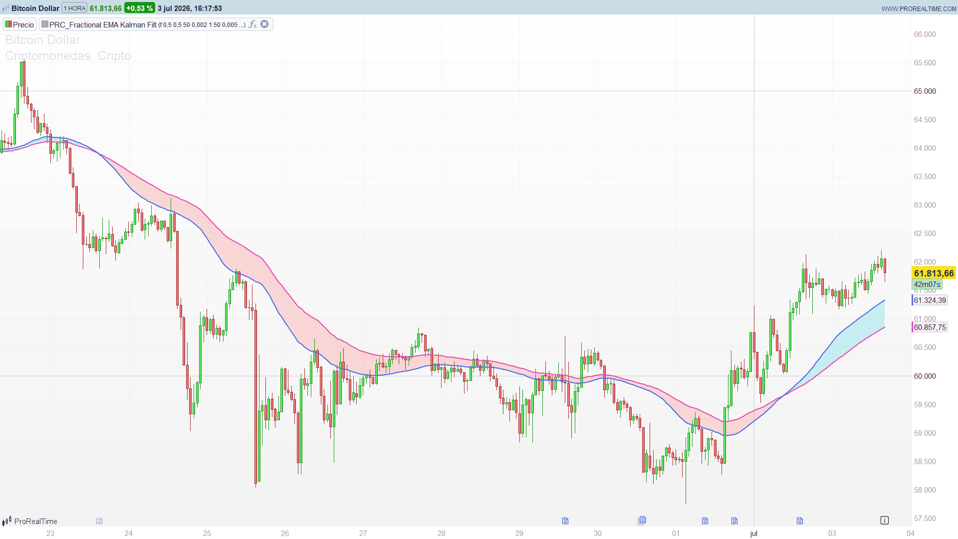
The indicator runs the whole machine twice with identical structure and different process-noise multipliers: a base version (q = 0.002, slower, the reference line) and a fast version (q = 0.005, more responsive). Each output gets a final short EMA (3 and 5 periods) to remove micro-jitter. The pair behaves like a moving-average crossover system, except both lines adapt to volatility and carry far less lag than averages of comparable smoothness. The area between them is filled aqua when the fast filter is above the base (bullish pressure) and red when below (bearish pressure).

How to Read the Indicator

1. Aqua fill (fast above base) — upward pressure; the recent regime is pulling the responsive filter above the slow reference.
2. Red fill (fast below base) — downward pressure; the mirror situation.
3. Fill colour flips are the discrete signal of the indicator — an adaptive, low-lag analogue of a moving-average crossover.
4. Width of the fill measures the strength of the move: a widening band means the fast filter is escaping from the base (acceleration); a narrowing band warns of exhaustion before the actual cross.
5. Slope of the base line gives the background bias; flips against a steep base line are more often noise, flips confirmed by the base line turning are regime changes.
6. The optional fractional EMA (hidden by default) shows the raw anticipative measurement with a purple shading of its one-bar displacement — useful to appreciate how much noise the Kalman stage is absorbing.

Practical Applications

1. Trend following with less lag. Use the fill colour as the direction filter for your entries; the adaptive gain means the lines flatten in ranges instead of whipsawing like fixed-length averages.
2. Crossover system. fast crosses over base / crosses under are natural long/short triggers, and translate directly into a ProScreener or a ProOrder condition.
3. Pullback timing. In an established aqua regime, price returning to the base line while the fill stays aqua is a low-lag pullback entry; the band narrowing and re-widening confirms resumption.
4. Exhaustion warning. A band that narrows bar after bar while price still pushes highs flags a decelerating trend well before a classic MA cross would.
5. Volatility-aware smoothing for other tools. The adaptive Kalman block is generic: any series can replace the fractional EMA as measurement, giving you a self-tuning smoother for oscillators or spreads.

Indicator Configuration

• showema (0/1, default 0): plot the underlying fractional EMA with its lag shading.
• factor, factor2 (default 0.5, minimum 0.1): lengths of the two cascaded EMA passes. Below 1 the EMA anticipates; at 1 it returns raw price; above 1 it behaves like a normal EMA.
• rratiob / rratios (default 50): lookback of the measurement-noise baseline R for the base and fast filters.
• qratiob / qratios (default 0.002 / 0.005): process-noise multipliers — the main sensitivity dials. Higher = more responsive filter.
• rgateb / rgates (default 1.0): multiplier of the dynamic R floor; raise it to make the filters more skeptical of sudden variance spikes.
• qlen (default 5): short lookback of the Q estimate, common to both filters.
• Colours match the original: base line in magenta, fast line in blue, aqua/red trend fill at low opacity.

Code

//----------------------------------------------
//PRC_Fractional EMA Kalman Filter D7
//Original author: et20tradeview
//version = 0
//03.07.2026
//Iván González @ www.prorealcode.com
//Sharing ProRealTime knowledge
//----------------------------------------------
// Doble filtro de Kalman adaptativo (base + rapido) sobre una
// EMA fraccional en cascada (longitud < 1 = anticipativa).
// El relleno entre ambos Kalman marca la tendencia.
//----------------------------------------------
// === Inputs (exponer como variables del indicador) ===
src = customclose
showema = 0       // 1 = mostrar la EMA fraccional y su sombreado de retardo
factor = 0.5      // longitud EMA fraccional 1 (minimo 0.1; < 1 = anticipativa)
factor2 = 0.5     // longitud EMA fraccional 2 (segunda pasada)
rratiob = 50      // version base: lookback de R (incertidumbre de medida)
qratiob = 0.002   // version base: multiplicador de Q (ruido de proceso)
rgateb = 1.0      // version base: multiplicador del suelo dinamico de R
rratios = 50      // version rapida: lookback de R
qratios = 0.005   // version rapida: multiplicador de Q
rgates = 1.0      // version rapida: multiplicador del suelo dinamico de R
qlen = 5          // lookback corto de Q (comun a ambas versiones)
//----------------------------------------------
// === EMA fraccional en cascada ===
// alpha = 2/(n+1) con n < 1 da alpha > 1: la "EMA" extrapola
// (coeficiente negativo sobre el valor previo) y gana anticipacion
alpha1 = 2 / (max(factor, 0.1) + 1)
alpha2 = 2 / (max(factor2, 0.1) + 1)
// volatilidad de referencia para normalizar el residuo
volbase = max(averagetruerange[14](close), 0.000001)

if barindex <= 12 then
   fema1 = src
   fema2 = src
   kfb = src
   kfs = src
   pcovb = 1.0
   pcovs = 1.0
   rrawb = 1.0
   rraws = 1.0
   qrawb = 0.1
   qraws = 0.1
   smoothb = src
   smooths = src
else
   fema1 = alpha1 * src + (1 - alpha1) * fema1[1]
   fema2 = alpha2 * fema1 + (1 - alpha2) * fema2[1]
   //----------------------------------------------
   // === Varianza del residuo normalizada por ATR ===
   residb = fema2 - kfb[1]
   resids = fema2 - kfs[1]
   rvarb = (residb * residb) / (volbase * volbase)
   rvars = (resids * resids) / (volbase * volbase)
   // R = base larga de la varianza (RMA 50), Q = impulso corto (RMA 5)
   rrawb = rrawb[1] + (rvarb - rrawb[1]) / rratiob
   qrawb = qrawb[1] + (rvarb - qrawb[1]) / qlen
   rraws = rraws[1] + (rvars - rraws[1]) / rratios
   qraws = qraws[1] + (rvars - qraws[1]) / qlen
   //----------------------------------------------
   // === Kalman base ===
   qprocb = min(max(qrawb, 0.001), 10) * qratiob
   radaptb = max(rrawb, rvarb * rgateb)
   cpb = pcovb[1] + qprocb
   kgainb = cpb / (cpb + radaptb + 0.0000000001)
   kfb = kfb[1] + kgainb * (fema2 - kfb[1])
   pcovb = (1 - kgainb) * cpb
   // === Kalman rapido ===
   qprocs = min(max(qraws, 0.001), 10) * qratios
   radapts = max(rraws, rvars * rgates)
   cps = pcovs[1] + qprocs
   kgains = cps / (cps + radapts + 0.0000000001)
   kfs = kfs[1] + kgains * (fema2 - kfs[1])
   pcovs = (1 - kgains) * cps
   //----------------------------------------------
   // === Suavizado final anti-microtemblor (EMA 3 y EMA 5) ===
   smoothb = 0.5 * kfb + 0.5 * smoothb[1]
   smooths = kfs / 3 + 2 * smooths[1] / 3
endif
//----------------------------------------------
// === EMA fraccional opcional + sombreado de retardo ===
if showema = 1 then
   emaplot = fema2
   aema = 76
else
   emaplot = undefined
   aema = 0
endif
colorbetween(fema2, fema2[1], 105, 53, 156, aema)
//----------------------------------------------
// === Relleno tendencial entre ambos Kalman ===
if smooths > smoothb then
   fr = 0
   fg = 188
   fb = 212
else
   fr = 255
   fg = 82
   fb = 82
endif
colorbetween(smoothb, smooths, fr, fg, fb, 51)

return smoothb coloured(230, 65, 195) style(line, 2) as "Kalman base", smooths coloured(80, 100, 240) style(line, 2) as "Kalman fast", emaplot coloured(156, 39, 176, 76) as "Fractional EMA"