AI Predictive Flow for ProRealTime

Introduction

Most oscillators describe what price has already done. AI Predictive Flow, by Zeiierman, asks a different question: the last few bars look like something the market has done before, so what happened next on those occasions?

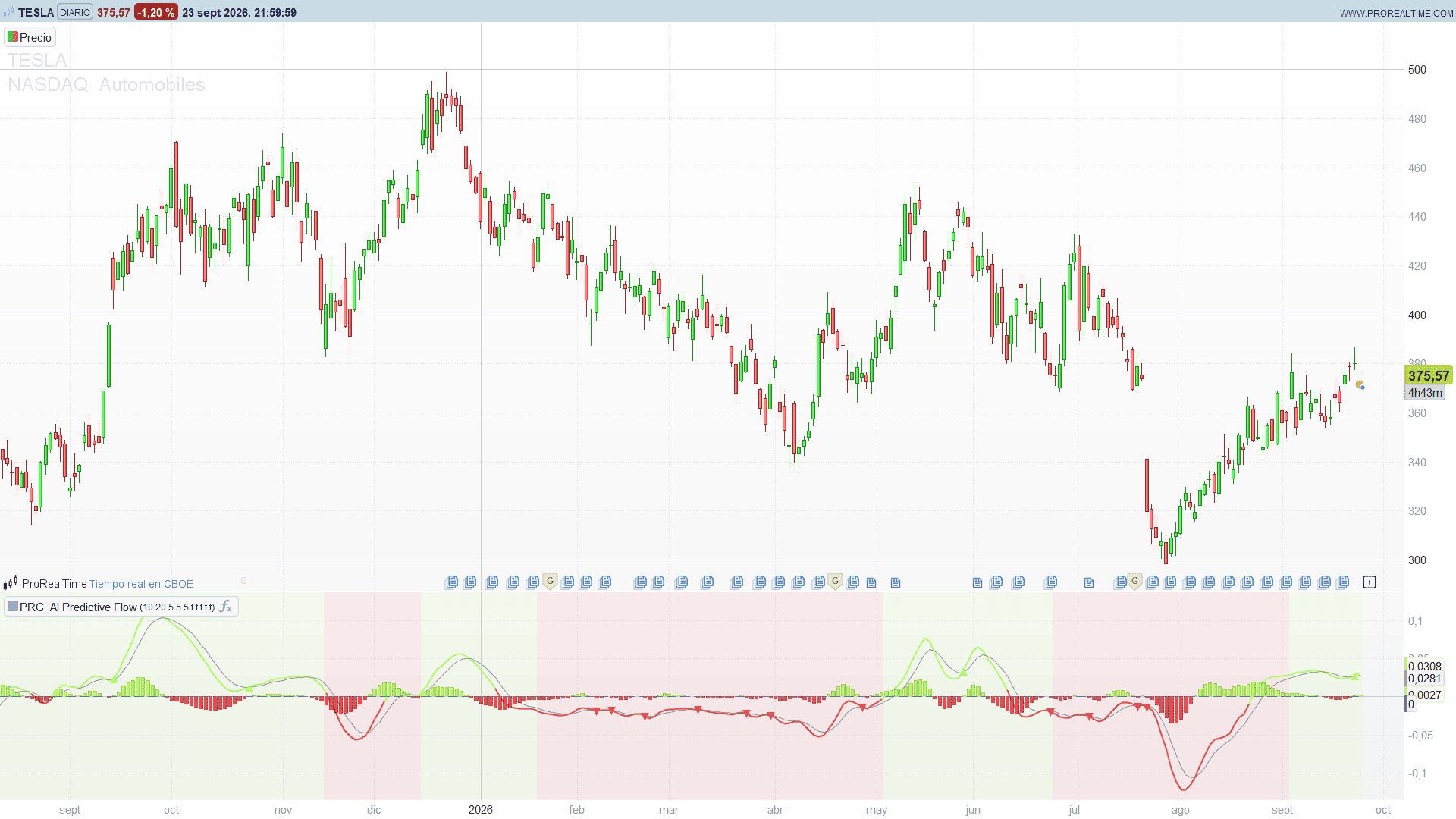
To answer it, the indicator keeps a rolling memory of recent price patterns together with what followed each one, finds the patterns most similar to the current one, and turns their outcomes into a forecast. The forecast is smoothed into an oscillator with a signal line and a histogram, and a background colour shows the predicted trend regime.

Theory Behind the Indicator

1. Describing a pattern

Each pattern is a window of patLen bars (10 by default), and every bar of the window is described by four features:

The log return of the bar
The 5 bar momentum, as a percentage
The RSI(14), centred on zero and scaled to the range -1 to +1
The distance between a 10 and a 30 period EMA, relative to price

2. A memory of patterns and outcomes

On every closed bar, the pattern that ended two bars ago is stored in memory together with its outcome: the log change of a 14 period EMA over the two bars that followed. That outcome is already known, so the model never looks into the future. The memory keeps the last mem patterns (20 by default) and forgets the oldest one when a new one comes in.

3. Finding the nearest neighbours

The current pattern, which ends on the last closed bar, is compared with every pattern in memory. The distance is the Euclidean distance over all bars and all four features, with equal weights. The kNb closest patterns (5 by default) are the nearest neighbours.

4. The forecast

The forecast is the sum of the outcomes of the nearest neighbours, each one weighted by 1 - distance / total distance, so that the closest matches count the most. A positive value means that similar patterns were followed by a rising average; a negative value, by a falling one.

5. From forecast to oscillator

The raw forecast is smoothed by an EMA (smth), then by a 3 period EMA to give the oscillator. A signal line is an EMA of the oscillator (sigLn), and the histogram is the difference between the two.

6. The predicted trend regime

The forecast is also projected onto price as a predicted line (the 14 period EMA moved by the forecast), with bands at two ATR(100) around it. When the upper band makes a new 30 bar high, the regime turns bullish; when the lower band makes a new 30 bar low, it turns bearish. The regime is shown as the background colour of the panel.

Key Features at a Glance

Nearest-neighbour (kNN) forecast built from a rolling memory of price patterns
Four features per bar: return, momentum, RSI and EMA spread
Oscillator, signal line and histogram, coloured by sign
Background colour for the predicted trend regime
Triangles on bullish and bearish crossovers of the oscillator and its signal line
The memory is updated only on closed bars, so the historical values do not repaint

How to Read the Indicator

Oscillator above zero (green): similar past patterns were followed by rising prices. Below zero (red): by falling prices.
Histogram: the distance between the oscillator and its signal line. Growing bars show the forecast is strengthening; shrinking bars show it is losing strength.
Bullish triangle: the oscillator crosses above its signal line while the signal is at or above zero, which is a confirmation inside a positive forecast. Bearish triangle: the opposite, crossing below with the signal at or below zero.
Background: the predicted trend regime. Green favours long setups, red favours short ones.

Practical Applications

Trend confirmation. Take trades in the direction of the background regime and use the oscillator crossing zero as the confirmation.
Pullback entries. In a green regime, a bullish triangle after a dip of the oscillator marks the point where the forecast turns up again.
Early warning. A shrinking histogram against the regime warns that the forecast is fading before the regime itself changes.

Indicator Configuration

patLen (default: 10, minimum 5): number of bars in each pattern. Higher values capture more structure but make the calculation heavier.
mem (default: 20, minimum 10): number of past patterns kept in memory. It is the main driver of the calculation time.
kNb (default: 5, from 1 to 20): number of nearest neighbours used in the forecast. Higher values give a smoother, slower forecast.
smth (default: 5): EMA smoothing of the raw forecast.
sigLn (default: 5): length of the signal line.
showOsc, showSig, showHist (default: 1): show or hide the oscillator, the signal line and the histogram.
showBg (default: 1): background colour of the predicted trend regime.
showMarks (default: 1): crossover triangles.

Apply the indicator in its own panel. The first forecasts appear after about 50 bars, once there is enough history to build the patterns. On the bar in progress, the indicator shows the forecast of the last closed bar and updates it when the bar closes.

Code

//---------------------------------------------------------------
//PRC_AI Predictive Flow (Zeiierman)
//version = 0
//24.09.2026
//Iván González @ www.prorealcode.com
//Author: Zeiierman
//Sharing ProRealTime knowledge
//--------------------------------------------------------------------//
// Apply it in its own panel (not on the price).

//----- Main settings
patLen = 10            // Pattern Length (min 5): bars of the pattern compared with past patterns
mem = 20               // Memory Size (min 10): historical patterns kept for the kNN search
kNb = 5                // Neighbors (1..20): nearest matches averaged into the prediction
smth = 5               // Prediction Smoothing (EMA of the raw prediction)
sigLn = 5              // Signal Length

//----- Style
showOsc = 1
showSig = 1
showHist = 1
showBg = 1             // predicted trend regime background
showMarks = 1          // bullish / bearish crossover markers

//----- Fixed internals
momLn = 5
rsiLn = 14
emaLn = 14
fLen = 10
sLen = 30
atrLn = 100
bandM = 2.0
regLn = 30
oscLn = 3
ahead = 2

patLen = max(5, round(patLen))
mem = max(10, round(mem))
kNb = min(20, max(1, round(kNb)))
tot = patLen + ahead
enoughBar = tot + max(momLn, sLen) + ahead + 5

//----- Base series
base = average[emaLn, 1](close)
atrV = averagetruerange[atrLn](close)
efS = average[fLen, 1](close)
esS = average[sLen, 1](close)
rsS = rsi[rsiLn](close)

//----- Pattern engine, once per CLOSED bar.
// Arrays are NOT rewound between ticks the way scalars are, so the memory is updated once
// per bar and only with data of a closed bar: on history each bar is processed on itself,
// and the live bar is processed when the next one opens, reading its data with offset 1.
// All the state of the engine lives in arrays for the same reason.
// $gState[0] = last processed bar, [1] = stored patterns, [2] = prediction,
// [3] = predicted line, [4] = prediction available (0/1)
IF barindex = 0 THEN
   $gState[0] = 0 - 1
   $gState[1] = 0
   $gState[2] = 0
   $gState[3] = 0
   $gState[4] = 0
ENDIF

FOR pss = 1 DOWNTO 0 DO
   ofs = pss
   doIt = 0
   IF ofs = 1 AND barindex >= 1 AND $gState[0] < barindex - 1 THEN
      doIt = 1
   ENDIF
   IF ofs = 0 AND NOT islastbarupdate AND $gState[0] < barindex THEN
      doIt = 1
   ENDIF
   IF doIt = 1 THEN
      $gState[0] = barindex - ofs
      IF barindex - ofs > enoughBar THEN
         // outcome of the pattern that ended "ahead" bars ago
         yv = log(base[ofs]) - log(base[ofs + ahead])
         nR = $gState[1]
         // memory full: drop the oldest pattern (row 0) and its outcome
         IF nR >= mem THEN
            FOR rR = 0 TO mem - 2 DO
               FOR jC = 0 TO patLen - 1 DO
                  $m1[rR * patLen + jC] = $m1[(rR + 1) * patLen + jC]
                  $m2[rR * patLen + jC] = $m2[(rR + 1) * patLen + jC]
                  $m3[rR * patLen + jC] = $m3[(rR + 1) * patLen + jC]
                  $m4[rR * patLen + jC] = $m4[(rR + 1) * patLen + jC]
               NEXT
               $yOut[rR] = $yOut[rR + 1]
            NEXT
            nR = mem - 1
         ENDIF
         // features: wh = 0 -> stored pattern (ends "ahead" bars ago), wh = 1 -> current pattern
         FOR iP = 0 TO patLen - 1 DO
            FOR wh = 0 TO 1 DO
               IF wh = 0 THEN
                  sh = tot - 1 - iP + ofs
               ELSE
                  sh = patLen - 1 - iP + ofs
               ENDIF
               cF = close[sh]
               c1F = close[sh + 1]
               cmF = close[sh + momLn]
               IF c1F <> 0 THEN
                  v1 = log(cF / c1F)
               ELSE
                  v1 = 0
               ENDIF
               IF cmF <> 0 THEN
                  v2 = (cF - cmF) / cmF
               ELSE
                  v2 = 0
               ENDIF
               v3 = (rsS[sh] - 50) / 50
               IF cF <> 0 THEN
                  v4 = (efS[sh] - esS[sh]) / cF
               ELSE
                  v4 = 0
               ENDIF
               IF wh = 0 THEN
                  $m1[nR * patLen + iP] = v1
                  $m2[nR * patLen + iP] = v2
                  $m3[nR * patLen + iP] = v3
                  $m4[nR * patLen + iP] = v4
               ELSE
                  $f1[iP] = v1
                  $f2[iP] = v2
                  $f3[iP] = v3
                  $f4[iP] = v4
               ENDIF
            NEXT
         NEXT
         $yOut[nR] = yv
         nR = nR + 1
         $gState[1] = nR
         // distance from the current pattern to every stored pattern
         FOR rR = 0 TO nR - 1 DO
            sD = 0
            FOR jC = 0 TO patLen - 1 DO
               d1 = $f1[jC] - $m1[rR * patLen + jC]
               d2 = $f2[jC] - $m2[rR * patLen + jC]
               d3 = $f3[jC] - $m3[rR * patLen + jC]
               d4 = $f4[jC] - $m4[rR * patLen + jC]
               sD = sD + d1 * d1 * 0.25 + d2 * d2 * 0.25 + d3 * d3 * 0.25 + d4 * d4 * 0.25
            NEXT
            $dst[rR] = sqrt(sD)
            $usd[rR] = 0
         NEXT
         // k nearest neighbours, closest first (ties: oldest pattern first)
         useN = min(kNb, nR)
         sumD = 0
         FOR qN = 0 TO useN - 1 DO
            best = 0 - 1
            FOR rR = 0 TO nR - 1 DO
               IF $usd[rR] = 0 THEN
                  IF best < 0 THEN
                     best = rR
                  ELSIF $dst[rR] < $dst[best] THEN
                     best = rR
                  ENDIF
               ENDIF
            NEXT
            $usd[best] = 1
            $sel[qN] = best
            sumD = sumD + $dst[best]
         NEXT
         avgP = 0
         FOR qN = 0 TO useN - 1 DO
            idxN = $sel[qN]
            dN = $dst[idxN]
            wN = 1
            IF useN > 1 AND sumD <> 0 THEN
               wN = 1 - dN / sumD
            ENDIF
            avgP = avgP + $yOut[idxN] * wN
         NEXT
         $gState[2] = avgP
         $gState[3] = base[ofs] + base[ofs] * (exp(avgP) - 1)
         $gState[4] = 1
      ENDIF
   ENDIF
NEXT

predOk = $gState[4]
pred = $gState[2]
predLine = $gState[3]

//----- Smoothing: EMAs seeded with the simple average of their first values
once nP = 0
once sP = 0
once predE = 0
once nO = 0
once sO = 0
once oscE = 0
once nS = 0
once sS = 0
once sigE = 0
aP = 2 / (smth + 1)
aO = 2 / (oscLn + 1)
aS2 = 2 / (sigLn + 1)
IF predOk = 1 THEN
   nP = nP + 1
   IF nP <= smth THEN
      sP = sP + pred
   ENDIF
   IF nP = smth THEN
      predE = sP / smth
   ELSIF nP > smth THEN
      predE = aP * pred + (1 - aP) * predE
   ENDIF
   IF nP >= smth THEN
      nO = nO + 1
      IF nO <= oscLn THEN
         sO = sO + predE
      ENDIF
      IF nO = oscLn THEN
         oscE = sO / oscLn
      ELSIF nO > oscLn THEN
         oscE = aO * predE + (1 - aO) * oscE
      ENDIF
      IF nO >= oscLn THEN
         nS = nS + 1
         IF nS <= sigLn THEN
            sS = sS + oscE
         ENDIF
         IF nS = sigLn THEN
            sigE = sS / sigLn
         ELSIF nS > sigLn THEN
            sigE = aS2 * oscE + (1 - aS2) * sigE
         ENDIF
      ENDIF
   ENDIF
ENDIF

oscOk = 0
IF nO >= oscLn THEN
   oscOk = 1
ENDIF
sigOk = 0
IF nS >= sigLn THEN
   sigOk = 1
ENDIF

//----- Predicted trend regime: new high / low of the ATR bands around the predicted line
once trendUp = 0
IF predOk = 1 THEN
   hiRef = predLine + bandM * atrV
   loRef = predLine - bandM * atrV
ELSE
   hiRef = 0
   loRef = 0
ENDIF
hiMax = highest[regLn](hiRef)
loMin = lowest[regLn](loRef)
// the window only counts once it holds regLn bars with a prediction
IF predOk = 1 AND nP >= regLn THEN
   IF hiMax = hiRef THEN
      trendUp = 1
   ENDIF
   IF loMin = loRef THEN
      trendUp = 0
   ENDIF
ENDIF

//----- Oscillator, signal and histogram
IF oscOk = 1 THEN
   osc = oscE
ELSE
   osc = undefined
ENDIF
IF sigOk = 1 THEN
   sig = sigE
   hist = oscE - sigE
ELSE
   sig = undefined
   hist = undefined
ENDIF

IF osc >= 0 THEN
   oR1 = 175
   oG1 = 255
   oB1 = 105
ELSE
   oR1 = 255
   oG1 = 71
   oB1 = 80
ENDIF
IF hist >= 0 THEN
   hR1 = 175
   hG1 = 255
   hB1 = 105
ELSE
   hR1 = 255
   hG1 = 71
   hB1 = 80
ENDIF
oscA = 255 * showOsc
sigA = 204 * showSig
histA = 204 * showHist

//----- Background of the predicted regime
IF showBg = 1 THEN
   IF trendUp = 1 THEN
      BACKGROUNDCOLOR(175, 255, 105, 20)
   ELSE
      BACKGROUNDCOLOR(255, 71, 80, 20)
   ENDIF
ENDIF

//----- Crossover markers (on the oscillator: a panel has no fixed top/bottom anchor)
IF showMarks = 1 AND sigOk = 1 AND sigOk[1] = 1 THEN
   IF osc crosses over sig AND sig >= 0 THEN
      DRAWTEXT("▲", barindex, osc) COLOURED(175, 255, 105)
   ENDIF
   IF osc crosses under sig AND sig <= 0 THEN
      DRAWTEXT("▼", barindex, osc) COLOURED(255, 71, 80)
   ENDIF
ENDIF

RETURN osc COLOURED(oR1, oG1, oB1, oscA) STYLE(line, 2) AS "Osc", sig COLOURED(120, 123, 134, sigA) AS "Signal", hist COLOURED(hR1, hG1, hB1, histA) STYLE(histogram) AS "Hist", 0 COLOURED(120, 123, 134) STYLE(dottedline2) AS "Zero"

Conclusion

AI Predictive Flow brings a simple machine learning idea to a familiar format: instead of a fixed formula, the oscillator is driven by what happened after the most similar patterns in the recent past. It adapts as the memory rolls forward, and it can be read like any other momentum oscillator.

AI Predictive Flow