

Trading Systems (ProBacktest & ProOrder)
Introduction to programming trading systems in ProRealTime
ProRealTime’s programming tool allows you to create customized investment strategies. Trading systems can be coded directly or generated via the assisted creation module (no coding required).
There are two ways to run your systems:
- As backtests, to test their performance on the historical data of a value
- As an automatic trading system, from the ProOrder module: orders are placed in real time from a trading or PaperTrading account.
Trading systems are programmed using the ProBuilder programming language, already used to create customized indicators in ProRealTime. New instructions have been added which apply exclusively to the creation of trading systems. Trading system programming includes instructions for position taking, stops and risk management for each system according to customized conditions such as :
- Indicators supplied with your platform or indicators you have programmed yourself
- Past performance of your trading system
- Your last orders
The results of the execution of a trading system are presented in the form of :
- “Equity Curve”, which graphically shows the evolution of your system’s gains/losses on the corresponding instrument.
- Position histogram (green for buying, red for short selling). No bar is shown if there is no transaction in progress.
- Detailed report, showing general system statistics for the corresponding instrument, over the selected runtime period.
In the case of a backtest, you can also optimize the variables in your system. In this way, you can select the combination of variables giving the best results over the instrument and study period.
In automatic trading, orders placed by the trading systems appear both in your PaperTrading portfolio and in the order list. Gains or losses realized by your systems are also reported in the portfolio.
This manual is organized as follows: the first part explains how to create and edit a trading system. The second part describes the ProBuilder instructions to be used for programming. The third part describes how to simulate systems with ProBacktest. Finally, the fourth part describes how to run systems in automatic trading mode. The appendices at the end of the manual give several examples of results and code displays, as well as a ProBuilder language glossary.
For beginners or those unfamiliar with programming, we recommend watching the video “Create, backtest and run automatic trading systems with ProRealTime“.
The information presented in this manual is solely intended to help you code or test your own trading systems. It is not intended as investment advice.
If you have any further questions about how ProBacktest works, you can ask our ProRealTime community on the ProRealCode forum, where you’ll also find online documentation with numerous examples.
Wishing you every success, we wish you happy reading!
Introduction
Access to trading system programming
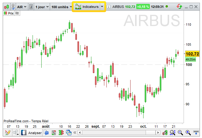
The window for creating trading systems is available from the “Indicators” button at the top1 of each of your ProRealTime charts.
You can also access it directly from your “View” menu1:
[1] Since ProRealTime version 12
By default, the management window opens on the “Indicators” tab. Go to the second tab, “ProBacktest & Automatic Trading”. You will then be able to :
- Access the list of existing systems (predefined or customized)
- Create a new system, then apply it to the value of your choice
- Modify, delete or duplicate an existing system
- Import or export systems
- Add your codes purchased on the ProRealCode Marketplace
The window for creating trading systems
The window for creating trading systems consists of two main areas:
- The creation area (assisted or programmed) on the left of the window.
- The application area on the right, which includes the ProBacktest tab for system simulation and the ProOrder tab for automatic trading. ProBacktest settings are described in detail in section 3 of this manual.
The creation area allows you to :
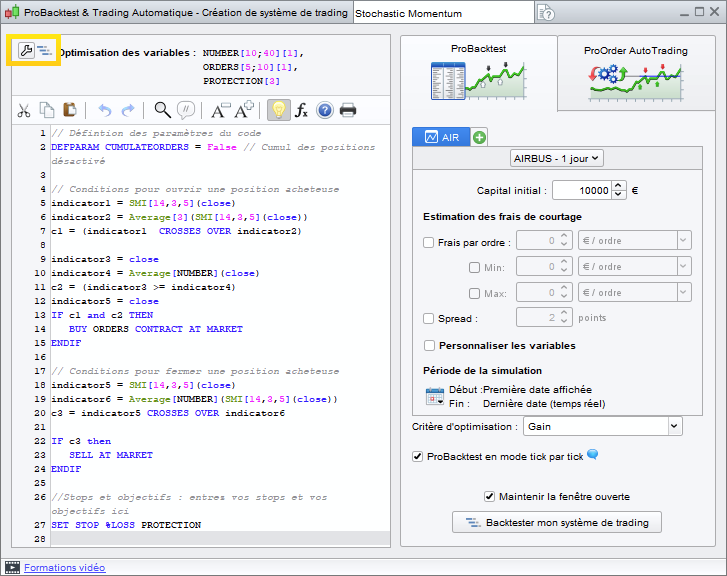
- Program a trading system directly into the text box.
- Use the “Insert Function” button, which opens a new window with a library of available functions to help you with programming. You’ll also find explanations related to the selected command or function.
Example:
Let’s use the function library by clicking on “Insert Function”.
Go to the “ProBacktest commands” section and click on “BUY“, then click on the “Add” button. The command will now be added to the programming area.
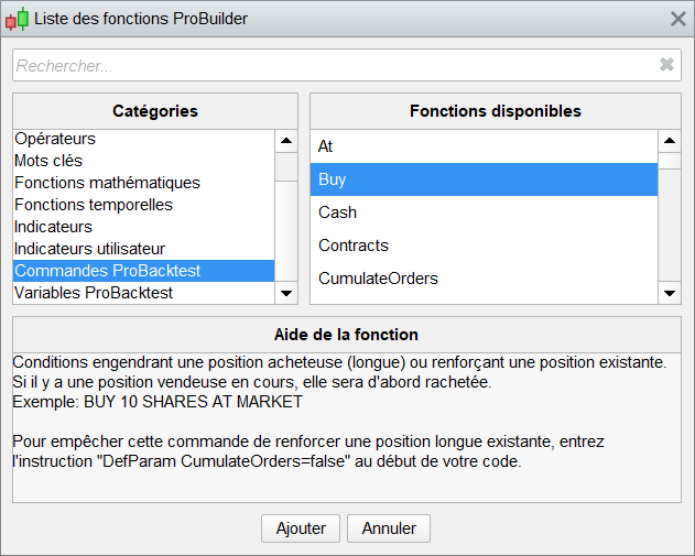
Let’s try to create a complete line of code. Let’s suppose, for example, that we want to buy 10 shares at market price.
Proceed as above to retrieve the “SHARES“, “AT” and “MARKET” instructions in this order (separate each word with a space).
You then receive the instruction “BUY 10 SHARES AT MARKET“, which commands the purchase of 10 shares at the market. The following section presents all the instructions available for programming trading systems.
Examples of complete system codes can be found in Appendix B of this manual.
Keyboard shortcuts
In ProRealTime version 12, the window for creating trading systems has several practical functions that can be used via keyboard shortcuts:
- Select all (Ctrl+A): Selects all text in the code editor.
- Copy (Ctrl + C) : Copies selected text
- Paste (Ctrl + V) : Pastes copied text
- Undo (Ctrl + Z): Cancels the last action performed in the code editor
- Redo (Ctrl + Y): Redoes the last action performed in the code editor
- Find / Replace (Ctrl + F): Find text in code editor / Replace text in code editor
- Comment / Uncomment (Ctrl + R): Comment the selected code / Uncomment the selected code: the commented code will be preceded by “//” or surrounded by “/* */” and colored gray. It will not be taken into account during code execution.
- Activate completion help (Ctrl + Space): Provides help on available features based on the beginning of the word the user is writing. It can be permanently activated/deactivated.
For MAC users, the same keyboard shortcuts can be used. In this case, simply replace the “Ctrl” key with the “Command” key.
Most of these shortcuts can also be used via a right-click in the code editor of the trading system creation window.
Programming trading systems
![]() Warning: The examples presented in this manual are for educational purposes only. You are free to choose your own trading criteria. All information presented is of a “general” nature and in no way represents personalized information or advice, or an inducement to buy or sell financial instruments. Past performance is no guarantee of future results, nor is it constant over time. Any trading system may expose you to a risk of loss greater than your initial investment.
Warning: The examples presented in this manual are for educational purposes only. You are free to choose your own trading criteria. All information presented is of a “general” nature and in no way represents personalized information or advice, or an inducement to buy or sell financial instruments. Past performance is no guarantee of future results, nor is it constant over time. Any trading system may expose you to a risk of loss greater than your initial investment.
Programming with ProBuilder
We strongly recommend reading the ProBuilder programming manual dedicated to indicator programming. This section covers additional ProBuilder instructions for trading systems.
ProBuilder is ProRealTime’s programming language. This language is very easy to use and offers a wide range of possibilities. It is based on the following principles:
- The basic unit is the candlestick, and the time unit is based on that of the current chart.
- A ProBuilder program and all its sub-functions are re-evaluated at the close of each candlestick, from the oldest to the most recent.
- All buy/sell instructions are calculated at the end of the current candlestick. They will therefore be triggered at the opening of the next candlestick at the earliest.
Market entries and exits
Different instructions apply depending on the direction of your position:
Long positions :
- BUY: securities purchase instruction (long entry)
- SELL: instruction to sell purchased securities (long exit)
The BUY instruction is used to open (or strengthen) a long market position. It is associated with the SELL instruction, which is used to close (or lighten) a long position. The SELL instruction has no effect if no long position is opened.
Short positions :
- SELLSHORT: short selling instruction (short entry)
- EXITSHORT: buyback instruction for securities sold short (short exit)
These two instructions work symmetrically with BUY and SELL. The EXITSHORT instruction has no effect if no short position is open.
It is not possible to take long and short positions on the same security at the same time. In practice, therefore, it is possible to close a long position with a SELLSHORT instruction, or to close a short position with a BUY command.
Note:
In automatic trading, remember to check that the maximum position size set at launch is not smaller than the position size your trading system will try to open (or reinforce), otherwise the order will not be transmitted and therefore not executed,
Each of these commands can be supplemented with the following items, which will be described in more detail later:
‘Order‘ ‘Quantity‘ AT ‘Type‘
Example:
BUY 1000 CASH AT MARKET or SELL 1 SHARE AT 1.56 LIMIT
Quantity
There are 2 ways of defining the quantity to be invested:
- SHARES corresponds to a unit of the instrument: “1 SHARE” represents 1 share, 1 warrant, 1 contract for futures, or 1 lot on Forex. SHARES can be replaced at any time by SHARE, CONTRACTS, PERPOINT, LOT or LOTS on any type of instrument. In the case of Forex, the quantity requested will be multiplied by the size of a lot. If the quantity is not specified, the default values are :
- 1 unit for a position entry (e.g. BUY AT MARKET places a “1” market order)
- The total quantity of the position for an output (e.g.: SELL AT MARKET closes the position completely).
- CASH corresponds to a transaction of a given amount (in € or $, for example) on shares only. The corresponding order quantity will then be calculated when the bar is closed (rounded down by default). Brokerage fees are not taken into account when calculating the quantity corresponding to the amount to be bought or sold.
Example: BUY 1000 CASH AT MARKET
You can use the ROUNDEDUP instruction to round this quantity up, or ROUNDEDDOWN to round this quantity down.
Example: BUY 1000 CASH ROUNDEDUP AT MARKET
Modes
Three order execution modes are available:
AT MARKET: The order will be placed at the market price at the opening of the next bar.
Example: BUY 1 SHARE AT MARKET
AT <price> LIMIT: A limit order will be placed at the specified price.
AT <price> STOP: A stop order will be placed at the indicated price.
Example: BUY 1 SHARE AT 10.5 LIMIT
Limit and stop orders at specific price levels are valid by default for one bar, from the opening of the next bar. If they have not been executed, they are cancelled when the next bar closes.
These orders are different from protection stops and profit limits (see next section). Protective stops and profit limits are linked to an already open position, and are valid until the position is closed.
These orders can be assimilated to market orders if conditions permit:
- If a BUY <quantity> AT <price> LIMIT order is placed above the current price, it will be treated as a market order.
- If a BUY <quantity> AT <price> STOP order is placed below the current price, it will be treated as a market order.
- If a SELLSHORT <quantity> AT <price> LIMIT order is placed below the current price, it will be treated as a market order.
- If a SELLSHORT <quantity> AT <price> STOP order is placed above the current price, it will be treated as a market order.
Example:
The following system involves buying 1 share at the market price when the RSI is in the oversold zone (RSI < 30) and prices are below the lower Bollinger band.
When the RSI is in the overbought zone (RSI > 70) and prices are above the upper Bollinger band, we sell.
[prc]
MyRSI = RSI[14](Close)
MyBollingerDown = BollingerDown[25](Close)
MyBollingerUp = BollingerUp[25](Close)
IF MyRSI < 30 AND Close < MyBollingerDown THEN
BUY 1 SHARE AT MARKET
ENDIF
IF MyRSI > 70 AND Close > MyBollingerUp THEN
SELL AT MARKET
ENDIF[/prc]
![]() You can define the validity period of your stop and limit orders.
You can define the validity period of your stop and limit orders.
The following example illustrates the use of certain variables to determine the validity of a limit order. Validity is expres-sed in number of bars. Here, the code places a limit order to buy at the closing price of the bar on which a moving ave-rage cross occurs. The limit order remains valid for 10 bars after the crossover. If it is not executed within this period, it will be cancelled.
Example:
// Define order validity period
ONCE NbBarLimit = 10
MM20 = Average[20](Close)
MM50 = Average[50](Close)
// If the MM20 crosses the MM50, we define 2 variables: “MyLimitBuy” and “MyIndex”, which respectively contain the current closing price and the index of the bar concerned by the crossing.
IF MM20 CROSSES OVER MM50 THEN
MyLimitBuy = Close
MyIndex = Barindex
ENDIF

IF BarIndex >= MyIndex + NbBarLimit THEN
MyLimitBuy = 0
ENDIF

// Places an order at the corresponding MyLimitBuy price, valid as long as this variable is greater than 0 and we are not in long position.
// Reminder: MyLimitBuy is greater than 0 for the 10 bars following the crossover.
IF MyLimitBuy > 0 AND NOT LongOnMarket THEN
BUY 1 SHARES AT MyLimitBuy LIMIT
ENDIF
If an order is not executed, it is possible to replace the expired limit buy order with a market buy order. The code block will allow you to do this if it is added after the previous block:
[prc]IF BarIndex = MyIndex + NbBarLimit AND NOT LongOnMarket THEN
BUY 1 SHARES AT MARKET
ENDIF[/prc]
Stops and Targets
ProBacktest also lets you define profit targets and protection stops. The syntax to use is as follows:
SET STOP <type> <value> or SET TARGET <type> <value>
Example:
SET STOP %LOSS 2 // Sets a stop loss of 2%.
Each variant is described below.
![]() It is important to distinguish between the different STOP commands:
It is important to distinguish between the different STOP commands:
- AT (price) STOP, is used to define an order with an execution threshold. This order is valid for one bar only.
- SET STOP LOSS (distance to price) / SET STOP (price), is used to define a protective stop, i.e. to exit an existing position. This order is valid until the position is closed.
Protective stops
Stop losses are used to limit the loss of a position. They can be defined relatively or absolutely:
SET STOP LOSS x : A protective stop is set at x units from the entry price.
SET STOP pLOSS x : A protective stop is set at x points from the entry price.
SET STOP %LOSS x : A protective stop is set at a level corresponding to a loss of x%.
SET STOP $LOSS x : A protective stop is set at a level corresponding to a loss of x€ or $ (instrument currency), excluding brokerage fees.
Protective stops can also be placed at the position’s entry price, making it possible to secure a position by preventing any loss (excluding brokerage fees):
SET STOP BREAKEVEN: A protective stop is set at the position entry price.
Finally, protective stops can be placed to secure a gain when the position is currently winning. In this case, they are placed in the direction of the position’s gain. They can be defined relatively or absolutely:
SET STOP PROFIT x : A protective stop is set at x units of the entry price.
SET STOP pPROFIT x : A protective stop is set at x points from the entry price.
SET STOP %PROFIT x : A protective stop is set at a level corresponding to a gain of x%.
SET STOP $PROFIT x : A protective stop is set at a level corresponding to a gain of x€ or $ (instrument currency), excluding brokerage fees.
Finally, it is possible to define a stop directly at a defined price, so that the stop can be placed in the direction of a loss or gain for the position:
SET STOP PRICE x : A protective stop is set at price x on the instrument.
The direction (buy/sell) and quantity of the stop order are automatically adapted to the current position. A protective stop is necessarily linked to a given position. If no position is open, the associated protective stop will not be active.
To deactivate a stop, use one of the following instructions:
SET STOP LOSS 0, SET STOP [p/%/$]LOSS 0, SET STOP BREAKEVEN 0, SET STOP PROFIT 0, SET STOP [p/%/$]PROFIT 0, SET STOP PRICE 0
As with the STOP and LIMIT opening orders seen above, a protective stop placed on the wrong side of the price will automatically be transformed into a market order to close the position.
Target orders (limit)
These instructions allow you to exit a position when the gains reach the set target.
SET TARGET PROFIT x : A limit is set at x units of the position entry price.
SET TARGET pPROFIT >x : A limit is set at x points from the position entry price.
SET TARGET %PROFIT >x : A limit is set at a level corresponding to a gain of x%.
SET TARGET $PROFIT x : A limit is set at a level corresponding to a gain of x€ or $ (currency of the instrument), excluding brokerage fees.
In the event of a losing position, you can limit the loss with a limit placed at the entry price, which will allow you to exit the position without gain or loss (excluding brokerage fees):
SET TARGET BREAKEVEN: A limit is set at the position entry price.
It is also possible to limit losses when a position is currently losing. The limit is placed in the direction of the position’s loss:
SET TARGET LOSS x : A limit is set at x units of the position entry price.
SET TARGET pLOSS x : A limit is set at x points from the position entry price.
SET TARGET %LOSS x : A limit is set at a level corresponding to a loss of x%.
SET TARGET $LOSS x : A limit is set at a level corresponding to a loss of x€ or $ (currency of the instrument), excluding brokerage fees.
Finally, as with protective stops, it is possible to place a profit limit directly at a defined price:
SET TARGET PRICE x : A limit is placed on the instrument at a price of X.
The direction (buy/sell) and quantity of the target order are automatically adapted to the current position. A target order is necessarily linked to a given position. If no position is open, the associated target order will not be active.
To deactivate a profit limit in the code, you can use one of the following instructions:
SET TARGET PROFIT 0, SET TARGET [p/%/$)PROFIT 0, SET TARGET BREAKEVEN 0, SET TARGET LOSS 0, SET TARGET [p/%/$)LOSS 0, SET TARGET PRICE 0
Be careful when placing target orders: as with STOP and LIMIT opening orders and position protection stops, a target order placed on the wrong side of the price will automatically be transformed into a market order to close the position.
Follower stops
A trailing stop is a stop order whose execution level changes according to price movements. For long positions, the stop will follow the price rise. If the price subsequently falls, the stop level remains unchanged.
In the case of short positions, the opposite is true: the stop will follow price falls, but will remain fixed in the event of a price rise.
Based on the same principle as protective stops, trailing stops can be defined relatively or absolutely:
SET STOP TRAILING y : A trailing stop is set at y units from the position entry price.
SET STOP pTRAILING y : A trailing stop is set at y points from the position entry price.
SET STOP %TRAILING y : A trailing stop is set at an initial level corresponding to a loss of y%.
SET STOP $TRAILING y : A trailing stop is set at an initial level corresponding to a loss of y€ or $ (instrument currency), excluding brokerage fees.
The direction and quantity of the trailing stop order are automatically adapted to the current position. A trailing stop is necessarily linked to a given position. If no position is open, the associated trailing stop will not be active.
If the position quantity changes (e.g. the position is strengthened), the stop threshold is reset.
To disable a trailing stop in the code, you can use one of the following instructions:
SET STOP TRAILING 0, SET STOP pTRAILING 0, SET STOP %TRAILING 0, SET STOP $TRAILING 0
Example:
You enter a position on the DAX future at a level of 6000 points and place a trailing stop at 50 points:
SET STOP pTRAILING 50
The stop is initially set at 5950. If the price rises to 6010 and then falls to 5980, the stop will rise by 10 points to 5960 and remain there until the price exceeds 6010. It will then be triggered if the price reaches 5960.
Using “Set Target / Set Stop” with an “IF” conditional instruction
You can modify the behavior of protection stops or profit limits in your code by adding custom conditions. The “IF” command can then be used.
Example:
// Place a stop loss of 10% if the gain of the previous position is at least 10%. Otherwise, place a stop loss of 5%.
IF PositionPerf(1)> 0.1 THEN
SET STOP %LOSS 10
ELSE
SET STOP %LOSS 5
ENDIF
Multi-level stops and limits
As a general rule, only one “Set Stop” instruction and one “Set Target” instruction can be entered and retained within a code. If your code contains several successive “Set Stop” or “Set Target” instructions, only the last command entered will be retained.
Multi-level stops can be used for backtesting and automatic trading on our PaperTrading module only.
Multi-level stops make it possible to combine a classic stop and a trailing stop on a position at the same time. The closer of the two stops is actually placed on the market, with the possibility of the trailing stop automatically taking the place of the classic stop according to market movements.
Example:
SET STOP %LOSS 10 // Set a 10% stop loss
SET TARGET PROFIT 50 // Set a profit limit of 50 units
SET TARGET %PROFIT 5 // Replaces the last profit limit with a profit limit of 5%.
SET STOP %TRAILING 2 // Replaces the last stop loss by a trailing stop of 2%.
However, it is possible to combine fixed and trailing stops, or stop-loss and trailing stops. A unique instruction has been developed for this purpose:
|
SET STOP |
<Mode> <value> | <TrailingType> <value> | ||
| threshold |
trailing |
Mode: LOSS, pLOSS, %LOSS, $LOSS
TrailingType: TRAILING, pTRAILING, %TRAILING, $TRAILING
This instruction will therefore take the form :
SET STOP[LOSS/pLOSS/$LOSS/%LOSS] <value> [TRAILING/pTRAILING/$TRAILING/%TRAILING] <value>
Examples of use:
SET STOP LOSS x TRAILING y : A protective stop is set at x units from the position entry price. Following a price change, if the difference between the trailing stop and the current price is less than the difference between the protective stop and the current price, then the protective stop becomes a trailing stop of y units.
SET STOP LOSS x pTRAILING y : A protective stop is set at x units from the entry price. Following a price change, if the difference between the trailing stop and the current price is less than the difference between the protective stop and the current price, then the protective stop becomes a trailing stop of y points.
SET STOP LOSS x $TRAILING y : A protective stop is set at x units from the entry price. Following a price variation, if the difference between the trailing stop and the current price is less than the difference between the protective stop and the current price, then the protective stop becomes a trailing stop of y € or $ (currency of the instrument).
SET STOP LOSS x %TRAILING y : A protective stop is set at x units from the position entry price. Following a price change, if the difference between the trailing stop and the current price is less than the difference between the protective stop and the current price, then the protective stop becomes a trailing stop by y%.
Example:
SET STOP LOSS x TRAILING y :
A protective stop is set at a price level x. If the set trailing stop level rises above x, the protective stop becomes a trailing stop of y units.
Suppose you enter a position on the DAX at 6500. The following code will place a protective stop 20 points from your entry level. This stop will become a trailing stop if the price rises above 6530.
SET STOP LOSS 20 TRAILING 50
The following charts illustrate the example: The stop is set at 20 points from the opening price, i.e. 6480.
If the price reaches 6530 (= 6500 + (50-20)), the stop becomes a trailing stop with a 50-point spread.
If the share price rises (here, it has risen to 6535), the trailing stop also rises: to 6485.
Clarification of the use of points or units for stop distances and limits
The size of the point varies according to the type of instrument, while the size of a unit (price variation of 1 on the chart) is of course always fixed. Depending on your code, and the instruments to which it is applied, it may be preferable to use distances in points or units. Example:
On the Eurodollar (EURUSD), 1 point = 1 pip = 0.0001
On index futures (DAX, FCE), 1 point = 1
On European interest rate futures, 1 point = 0.01 (one basis point)
This information is available in our language using the keyword POINTSIZE.
Stop a trading system with QUIT
The “QUIT” instruction allows you to stop a trading system. The stop takes effect when the current bar is closed. Pending orders are cancelled, and all open positions are closed if your platform’s trading parameters so require. This allows you to easily stop a trading system in the event of large losses or after a certain date, for example.
Example:
IF Date> 20250101 THEN // Stop the strategy after January 1, 2025.
QUIT
ENDIF
Position monitoring
State variables
The 3 variables used to manage the state of a trading system are :
ONMARKET: 1 if you have open positions, 0 otherwise
LONGONMARKET: 1 if you have open long positions, 0 otherwise
SHORTONMARKET: 1 if you have open short positions, 0 otherwise
They can be used with square brackets. For example, ONMARKET[1] is 1 if positions were open at the close of the previous bar, 0 otherwise.
These variables are often used in conjunction with “IF” type instructions before an entry in position :
Example:
// We define the MACD
Indicator1 = MACD[12,26,9](Close)
// Observe changes in sign of the MACD Histogram
c1 = (Indicator1 CROSSES OVER 0)
// Buy: If there is no current long position and MACD >0 , buy 3 shares or lots.
IF NOT LONGONMARKET AND c1 THEN
BUY 3 SHARES AT MARKET
ENDIF
Position size variables
These 3 variables give the quantity of the current position:
COUNTOFPOSITION: gives position size (in lots, shares or contracts). Positive if long position, negative if short position.
COUNTOFLONGSHARES: gives position size (in lots, shares or contracts) if a long position is in progress, 0 otherwise.
COUNTOFSHORTSHARES: gives position size (in lots, shares or contracts) if a short position is open, 0 otherwise.
As with instructions checking position status, these commands are generally used with “IF” instructions before entering position, and may include square brackets.
![]() A reminder about state variables: the code is evaluated at the end of the candlestick, and orders are placed at the opening of the next bar, In the following code, the “long” variable will not be equal to 1 at the close of the first candlestick, but only at the close of the second candlestick. This is because the first buy order was placed at the opening of the second candlestick.
A reminder about state variables: the code is evaluated at the end of the candlestick, and orders are placed at the opening of the next bar, In the following code, the “long” variable will not be equal to 1 at the close of the first candlestick, but only at the close of the second candlestick. This is because the first buy order was placed at the opening of the second candlestick.
BUY 1 SHARE AT MARKET
IF LONGONMARKET THEN
long = 1
ENDIF
LongTriggered
The LONGTRIGGERED[n] command is used to find out whether a long position has been opened on candlestick n.
LongTriggered[nth previous candlestick].
Note: It is possible to use LongTriggered without associating it with a bar number defined between brackets. In this case, the program will consider the candlestick bar currently being calculated, as if you had written : LongTriggered= LongTriggered[0]
Example:
//Only reopen a long position if we haven’t had a position open/close on the same candlestick:
IF NOT LONGONMARKET AND LongTriggered= 0 THEN
BUY AT MARKET
ENDIF
ShortTriggered
The SHORTTRIGGERED[n] command is used to find out whether a short position has been opened on candlestick n.
ShortTriggered[nth previous candlestick].
Note: It is possible to use ShortTriggered without associating it with a bar number defined between brackets. In this case, the program will consider the candlestick bar currently being calculated, as if you had written: ShortTriggered= ShortTriggered[0]
Example:
//We only reopen a short sale if we haven’t had a position open/close on the same candlestick:
IF NOT SHORTONMARKET AND ShortTriggered =  0 THEN
SELLSHORT AT MARKET
ENDIF
TradeIndex
The TRADEINDEX(n) command accesses the bar of the nth order previously executed.
TRADEINDEX(nth preceding order)
Note: It is possible to use TradeIndex without associating it with a bar number defined in brackets. In this case, the program will consider the bar of the last order placed, as if you had written: TradeIndex= TradeIndex(1). TradeIndex is generally associated with Barindex.
Example:
// If you have been in position for at least 3 bars :
IF LONGONMARKET AND (BarIndex – TradeIndex)>= 3 THEN
SELL AT MARKET
ENDIF
TradePrice
The TRADEPRICE(n) command is used to call up the price at which a transaction has been executed. Its syntax is as follows:
TRADEPRICE(nth preceding order)
You can specify the order to which you are referring in brackets. If you do not specify the order following TradePrice, the program will consider the price of the last order executed, as if you had written: TradePrice= TradePrice(1)
Example:
// If the closing price is higher than the execution price of the last transaction plus 2%.
IF LONGONMARKET AND CLOSE> 1.02 * TRADEPRICE THEN
SELL AT MARKET
ENDIF
PositionPerf
This command gives access to :
- The performance (ratio of gains to costs of the position) of the nth last position closed, if n >0 (excluding brokerage fees).
- Performance (ratio of gains to costs of position) of current position, if n=0 (excluding brokerage fees)
Its syntax is as follows:
POSITIONPERF(nth previous position)
If n is not entered, the program will assume that n=0: PositionPerf= PositionPerf(0)
Example:
// Buy if the previous trade made at least 20% profit
IF NOT ONMARKET AND PositionPerf(1)> 0.2 THEN
BUY 1000 CASH AT MARKET
ENDIF
PositionPrice
The PositionPrice command displays the average price of the current position.
POSITIONPRICE
The average price of a position is defined as the sum of the entry prices weighted by the quantity of each order. Only position reinforcements will influence the average price of the position.
This instruction can be used with square brackets (offset): POSITIONPRICE[1] returns the value PositionPrice had at the close of the previous candlestick.
Example:
You buy a share at €5, then strengthen your position by buying a share at €10, then another at €15.
The PositionPrice is therefore (5+10+15) / 3 = 10€.
You then decide to reduce your position by selling a share for €20. The value of PositionPrice will remain unchanged at €10.
StrategyProfit
This instruction returns the gains or losses (absolute, in the currency of the instrument and excluding brokerage fees) actually realized since the start of the trading system. Unrealized gains/losses are not taken into account.
It can be combined with the QUIT instruction to limit system losses.
STRATEGYPROFIT
You can also add square brackets: StrategyProfit[1], for example, will give the amount of profit at the close of the previous bar.
Example:
IF STRATEGYPROFIT < -500 THEN
QUIT
ENDIF
Note: As a reminder, your systems’ code is evaluated at the close of each candlestick. Using the example above, losses can exceed €500: for example, if a gap occurs, or if a sharp drop occurs within a single candlestick. It is therefore advisable to use STOP LOSS to protect losses on the position, and this code block to stop the system.
Definition of execution parameters for trading systems
Additional parameters can be defined using the DEFPARAM instruction.
![]() Reminder about DEFPARAM: they must always be placed at the beginning of your code.
Reminder about DEFPARAM: they must always be placed at the beginning of your code.
Cumulative orders in the same direction
The “CumulateOrders” parameter is used to authorize or prohibit the cumulation of orders, when entering a market position or reinforcing a position. By default, this parameter is active (“True”) when you create a new code directly by programming: with each new bar, the system will therefore be able to add a position to an existing position if the position entry conditions are verified. If you wish to enter the market with stop or limit orders, activate “CumulateOrders” to have several stops or limits active at the same time. To ensure that a system will not increase the size of an already open position, it is necessary to insert the following instruction at the very beginning of the code:
DEFPARAM CUMULATEORDERS = False
The DEFPARAM command remains active for the duration of your trading system’s runtime. It is not possible to change the order accumulation setting while the system is running.
Examples:
// This code will buy 1 share at each bar, with a maximum of 3 current positions.
DEFPARAM CUMULATEORDERS =  True
IF COUNTOFPOSITION <  3 THEN
BUY 1 SHARES AT MARKET
ENDIF
// This code will buy 1 share at the price of 2 and an additional share at the price of 3,
DEFPARAM CUMULATEORDERS =  True
IF COUNTOFPOSITION <  2 THEN
BUY 1 SHARES AT 2 LIMIT
BUY 1 SHARES AT 3 LIMIT
ENDIF
// This code will buy 5 shares once only
DEFPARAM CUMULATEORDERS =  False
BUY 5 SHARES AT MARKET
Several orders in the same direction can be placed simultaneously to exit the market, even when “CUMULATEORDERS” is set to “False“.
For example:
// This code will buy 5 shares. Up to 3 shares can be sold if the price crosses the MM40 on the downside, and the entire position is liquidated if a loss of at least 10% is realized.
DEFPARAM CUMULATEORDERS =  False
BUY 5 SHARES AT MARKET
IF Close CROSSES UNDER Average[40] THEN
SELL 3 SHARES AT MARKET
SET STOP %Trailing 10
ENDIF
Note on stops and limits when CUMULATEORDERS is active (“True“): It is always possible to place protective stops and profit limits while this parameter is active. In this case, the level of stop and limit orders will be based on the average entry level of your positions. Their levels will be recalculated each time the overall position size is modified.
For example:
If you buy a share at €10.00, place a 10% protective stop and a 150% profit limit, the initial levels of these orders will be : Stop at €9.00, limit at €25.00. If you buy a second share at €20.00, your average entry price will be €15. As a result, the new stop levels and limits will be : Stop at $13.50, limit at €37.50 (position taken as a whole).
Note on codes generated in “assisted creation” mode: CUMULATEORDERS is deactivated by default in codes generated in assisted creation mode (the instruction “DEFPARAM CUMULATEORDERS= False” is inserted at the start of the code).
Preload history
The DEFPARAM PRELOADBARS instruction defines the maximum number of bars preloaded before a trading system is started. This instruction is very useful when your system uses indicators that require a certain amount of history to be loaded in order to calculate. This parameter is set to 1000 by default. It cannot be less than 0 or greater than 10,000. The system needs to run a calculation on at least one historical candlestick in order to initialize your code on our servers.
Therefore, using DEFPARAM PRELOADBARS = 0 will have the same effect as DEFPARAM PRELOADBARS = 1, i.e. there will be a preloaded candlestick to launch your trading system.
The value entered for this parameter is a maximum, as preloading depends on the amount of history available for the selected instrument and time frame.
For example:
DEFPARAM PRELOADBARS= 300
a = (Close+ Open) / 2
IF Close CROSSES OVER Average[250](a) THEN
BUY 1 SHARE AT MARKET
ENDIF
Taking the example of a moving average with a period of 250, if the PRELOADBARS parameter is set to 300, the moving average will have sufficient data to calculate itself at system start-up. This will not be the case if the parameter is set to 200 (250>200).
As mentioned above, 300 is a maximum number. If fewer than 300 bars are available before system start-up, preloading will be based on the number of bars available.
Continuing with this example, the “BarIndex” of the first bar following system startup will equal 300. On the other hand, if no bar is preloaded, the “BarIndex” of the first bar following system startup will equal 1.
Warning: a variable assignment preceded by “ONCE” will be executed only once on the first reading of this line of code (including the history loaded with “PRELOADBARS“).
In the example below, the strategy will not place any orders (because tmp is at 1 during PRELOADBARS, and no orders can be placed during this period).
Example:
DEFPARAM PRELOADBARS =  200
ONCE tmp = 1
IF tmp = 1 THEN
BUY 1 SHARE AT MARKET
tmp = 0
ENDIF
FLATBEFORE and FLATAFTER
DEFPARAM FLATBEFORE HHMMSS=
DEFPARAM FLATAFTER= HHMMSS
HHMMSS is the detailed time, where HH stands for hours, MM for minutes and SS for seconds.
These instructions allow you to cancel any pending order, close any open position and prevent any additional orders from being added before the set time (in the case of FLATBEFORE) or after the set time (in the case of FLATAFTER) in the time zone defined for the strategy.
The value associated with the FLATBEFORE instruction must always be greater than the market opening time (or the start time of the custom schedule, if defined). The value associated with the FLATAFTER instruction must be less than the market closing time (or end of custom schedule if defined). Otherwise, these parameters simply have no effect. If the set time is not a multiple of the trading system’s main time unit (i.e. it occurs within an ongoing candlestick), then the DEFPARAM FLATAFTER instruction will take effect at the close of that candlestick. The DEFPARAM FLATBEFORE instruction, on the other hand, will be applied as soon as the candlestick preceding the bar containing the set time closes.
For example:
DEFPARAM FLATBEFORE= 093000 // Cancels any pending orders, closes any open positions and prevents the system from adding any additional orders before 09h30min00sec (in the strategy’s time zone).
DEFPARAM FLATAFTER= 160000 // Cancels any pending orders, closes any open positions and prevents the system from adding any additional orders after 16h00min00sec (in the strategy’s time zone)
Reinvest gains (backtests only)
DEFPARAM NOCASHUPDATE= True
If this option is activated, the available cash is not updated with gains, losses and brokerage fees.
Example:
Initial capital €10,000, with “NOCASHUPDATE = True”. The maximum investment will be limited to €10,000, regardless of gains or losses during the Backtest run.
Note:
Parameters defined using the DEFPARAM instruction must be defined at the beginning of the code (after any comments).
MinOrder and MaxOrder (backtests only)
DEFPARAM MINORDER = n
DEFPARAM MAXORDER = p
This option is used to block orders whose quantity (in lots, contracts or shares) is less than n or greater than p.
Example:
DEFPARAM MINORDER =  100
BUY 1000 CASH AT MARKET
If the last price of the instrument is above €10, the order quantity will be less than 100 and the order will not be sent.
Calling up indicators
ProRealTime indicators
All the functions you use to create your personal indicators are also available for creating your trading systems, including ProRealTime indicators (see glossary at the end of this manual for a complete list of functions).
Please also refer to the ProBuilder manual for more information on these functions.
The amount of history required to calculate an indicator depends on the nature of the indicator.
For example, it is generally considered that calculating an exponential moving average of N ExponentialAverage[n] periods requires 20*N bars to give an accurate result.
If the start date of a backtest is very close to the first date on the chart, the server provides additional history so that trading systems can display results from the very first bar.
Customized indicators
As with indicator programming, your system can call up custom indicators using the CALL instruction.
Example:
a,b = CALL “HistoMACD“[5,6] // 5 and 6 being the parameters passed as input to the HistoMACD function
To find out more about how to make the best use of CALL, please refer to the section on programming tips for trading systems.
Programming tips
The calculation time of a system depends on the complexity of the indicators used and the way they are called up. The following paragraph offers a few simple tips for optimizing your code.
Reduce the number of calls to ProRealTime indicators
If you use the same ProRealTime indicator several times in different calculations, don’t call it up again. Instead, always store the indicator in an intermediate variable:
| NON-OPTIMAL CODE | OPTIMAL CODE |
|
|
This advice also applies when you want to use the same indicator several times but with a different offset.
| NON-OPTIMAL CODE | OPTIMAL CODE |
|
|
Customized indicator calls
Calling up custom indicators via the CALL instruction is more time-consuming than calling up ProRealTime indicators. With ProRealTime indicators, we know in advance which calculations are required, and we have control over their execution. This is not the case with customized indicators, whose programming is specific to each user.
To improve a system’s execution speed, it is therefore important to optimize the use of the CALL instruction in its code.
Limit the number of identical calls:
As with ProRealTime indicators, it is advisable to limit the number of calls to custom indicators within a single code:
| NON-OPTIMAL CODE | OPTIMAL CODE |
|
|
ProBacktest – Trading system simulation
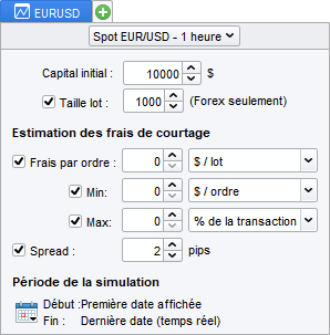
The “ProBacktest” tab in the trading system creation window is used to configure the brokerage parameters that will be used to simulate the system:
- Instrument(s)
- Graph for backtesting
- Initial capital
- Lot size (forex)
- Brokerage parameters
- Optimization variable model
- Simulation period
- Optimization criteria
Capital / Money Management
Initial capital
This section is used to enter the capital allocated to the trading system. The maximum investment allowed while the system is running depends on it.
While the backtest is running, brokerage fees as well as gains and losses will increase or decrease it (unless the NOCASHUPDATE parameter is activated). See Reinvesting gains for more details. The capital available for automatic trading systems corresponds to the capital available in the portfolio.
![]() If your trading system does not take any positions, consider increasing the Initial Capital amount.
If your trading system does not take any positions, consider increasing the Initial Capital amount.
Brokerage fees and spread
You can adjust these parameters to accurately reflect your broker’s fees. Any type of brokerage fee can be applied to any type of instrument. Possible fee types are :
- Fixed amount per order: fixed amount in instrument currency applied each time an order is executed. You can also specify a minimum or maximum value per order.
- Percentage: percentage of the transaction (in the currency of the instrument) applied each time an order is executed.
- Batch amount: fixed amount (in the currency of the instrument) applied per executed batch or contract.
- Lot size (Forex only): minimum size of a Forex order. Each order quantity used in BUY/SELL instructions is multiplied by the lot size.
- Spread (in points or pips): price difference between the best Bid and the best Ask.
Futures :
Brokerage fees are defined as commission per lot and per transaction.
Margin, or “Lot Deposit”, is the cash required to purchase a contract. The value of a point is automatically calculated by the platform according to the future concerned by the trading system.
Here are the point values for the main futures:
|
FUTURE NAME |
VALUE 1 POINT |
|
FCE CAC 40 |
10€ |
|
DAX |
25€ |
|
DJ Eurostoxx 50 |
10€ |
|
BUND |
10€ |
|
Euro FX |
12,5$ |
|
Mini S&P 500 |
50$ |
| Mini Nasdaq 100 |
20$ |
| Mini Dow |
5$ |
This information is available in our language using the keyword POINTVALUE.
Forex :
Brokerage parameters are used to define lot sizes and the spread to be applied to each order.
Example with EURUSD :
Batch size: 100,000
Spread: 2 pips
Margin: 5% (=Leverage x20)
The BUY 1 LOT AT MARKET instruction on EURUSD will buy a lot of 100,000, with a spread of 2 pips (i.e. 0.0002). As the leverage is 20 (5% margin), you need to own €5,000.
Actions :
Brokerage fees are defined as fees per order, in € or % of transaction. It is also possible to define a minimum brokerage fee per transaction.
On equities, position sizes and commitments per transaction are defined as a percentage of capital, or in the currency of the instrument. Risk Management can be used to limit the amount invested when placing an order, and to apply leverage.
Example:
- Brokerage fee per order: €10
- Margin: 20%.
With this configuration, each order placed can have a leverage of 5.
Variable optimization
In this section, you can choose to optimize variables. For a given instrument and time horizon, this function allows you to test different combinations of variables, to determine which give the best performance.
To find out more and see a concrete example, watch the video “Money management, stops and optimization“.
The result of the optimization is presented in an “Optimization Report”. You’ll see the statistics of the best combinations of variables tested, so you can determine which one you should use to make your trading system optimal.
Here is an example of a system with optimization of the periods of the n and m moving averages:
AVGm = ExponentialAverage[m](Close)
AVGn = ExponentialAverage[n](Close)
IF AVGm CROSSES OVER AVGn THEN
BUY 100 SHARES AT MARKET
ENDIF
IF AVGm CROSSES UNDER AVGn THEN
SELL 100 SHARES AT MARKET
ENDIF
Variables n and m can be defined by clicking on the “Add” button in the “Variable optimization” section.
![]()
The following window appears:

- “Name in program” represents the name the variable takes in our code (here n and m).
- “Fixed value” is used to set the variable to a defined value.
- “Min value”/”Max value” represent the limits between which the variable oscillates,
- “Step” represents the minimum interval between each value tested during optimization.
Here’s an example of an optimization report:

The example report shows 5 statistics for each combination of variables tested. These statistics are as follows:
- “Gain” refers to the capital gain realized by the trading system. This corresponds to the formula :
Profit = Final capital amount – Initial capital amount
This statistic provides an absolute assessment of the earnings potential of the defined system (for a given combination of variables and study period).
Note: the brokerage fees defined in the “Capital management” section are taken into account in this calculation.
- “%Gain” represents the profit or loss as a percentage. It corresponds to the formula :
%Gain = 100 x Profit / Initial capital amount
Indicates the relative performance of a system configured with the values of a given combination of variables.
- “Transactions” shows the number of positions opened during this system.
- “Win %” refers to the percentage of winning positions in the system. Mathematically, it is defined by :
% winning trades = (100 x Number of winning trades) / Number of trades
- “Average Gain” represents the average gain per position. This information is useful for determining the average efficiency of orders placed, especially when you don’t want to place many orders. It is defined by :
Average earnings per position = Earnings / Number of positions
Note: the optimal values of variables in a trading system may vary, for the same value, depending on the time units or history used.
Setting the backtest execution period
These fields allow you to define the start and end dates of your backtest. The amount of data used for a backtest is generally limited to the history displayed on the graph. You can increase this amount of history via the drop-down menu at the top left of each graph. It is necessary to load the amount of history you require before launching your backtest.
In the case of a backtest performed in “real time”, orders appear on the chart each time a signal is triggered (buy, sell, etc.). It is also possible to associate these orders with popups or sounds from the “Option/configure alerts and sounds” menu.
If an end date is set, positions still open on that date will be closed.
Note:
If your backtest takes a long time to run, you can reduce its execution period: calculation time is proportional to the length of the history.
After running a trading system, the following information is displayed:
- Evolution of the profit & loss curve at each candlestick
- Position trends
- Detailed report
To find out more about displaying backtest results, see Appendix A at the end of this document.
Tick by tick mode :
You can run your backtest in tick-by-tick mode to resolve execution sequence issues when two orders can be executed in the same candlestick.
![]()
Using this option can have an impact on the calculation time of your trading system. The greater the number of positions requiring verification, the greater the impact on your code’s calculation performance. To avoid excessive calculation times, a limit has been set on the number of positions that can be checked in tick-by-tick mode (500 by default, 2500 for premium platforms).
It should also be noted that the use of this option can have an impact on the position-taking results of your trading system, and thus modify its overall performance.
You can also use this option in combination with the backtest module’s optimization variables. When the option is checked, backtest will be able to count the number of conflicts between a STOP and TARGET instruction in the same candlestick.
So you’ll see a new column in your optimization report entitled “Mode tick”, representing the number of conflicts for each backtest.
After clicking on one of the lines in your optimization report, the associated backtest will be launched, resolving each conflict to find out which of your STOP and TARGET instructions was hit first, giving you more relevant results.
Note: the results displayed may differ between the optimization report and the backtest results, as the tick-by-tick mode is not applied directly during optimization, but only after opening the backtest.
Customize time slots for backtests
The “Time zones and time ranges” section of the “Settings” window lets you define customized time ranges for different markets.
Customized time slots: if you define reduced time slots for a market, only data falling within this time slot will be displayed on the charts (and therefore taken into account in ProBacktest). Please note that reduced time slots cannot be set to straddle two separate trading days. For example, on a 24-hour market, you can define a reduced time slot between 10:00 and 14:00, but it is not possible to define a time slot between 21:00 on the first day and 09:00 on the following day. If an order is supposed to be placed at the close of the last bar of the customized time slot, it will be placed at the opening of the first bar of the customized time slot on the following day.
The Dopen(x)/Dhigh(x)/Dlow(x)/Dclose(x) price constants on the current candlestick (x=0) take into account the custom time frames you’ve defined. They take official market data (without custom time frames) for previous candlesticks (x>0).
Using the option to apply these settings in daily and superior time units does not affect this behavior.
Notes on weekend data :
Some of the 24-hour markets offer the “Use intraday quotes to build daily candlesticks” option. This option is not taken into account by ProBacktest, which only uses daily candlesticks based on standard market hours.
Some markets include weekend data (e.g. Forex). For these markets, you can check a box to hide weekend data in the charts, via the “Options/Intraday chart time zones” menu. Weekend data are always taken into account for backtests. In Forex, Sunday data are included in the daily candlestick for Monday (there is no daily candlestick for Sunday). However, depending on the conditions set by your broker, this rule may differ, and Sunday may have its own daily candlestick.
Notes on custom time zones :
The code is always executed in the user’s time zone. This means that all time instructions (Time, FLATAFTER, FLATBEFORE) will take this time zone into account in their calculation. The user time zone is the time zone selected for the market to which the instrument belongs, and can be configured in the “Time zones and time ranges” section of the “Settings” window.
By default, the instrument’s time zone is that of your computer.
You can change a market’s time zone from the “Time zones and ranges” section of the “Settings” window. The next time the backtest is launched on an instrument from this market, the new time zone will be taken into account.
Example: On Vodafone (on the LSE, whose official time zone is GMT+1 daylight saving time or BST), I set my chart to Paris time (GMT+2 daylight saving time, or CET).
In 15 minutes, on the 11:45 London time (BST, GMT+1 in summer time) candlestick, the Time instruction will return 130000 (closing time of the 11:45 BST 15-minute candlestick: 12:00, transposed into CET time: 13:00).
The instructions concerned are all intraday time instructions:
- Time and its derivatives (Hour, Minute)
- Opentime and its derivatives (OpenHour, OpenMinute)
- FLATAFTER and FLATBEFORE
- IntradayBarIndex (reset to zero when the market opens in the user’s time zone)
Daily time instructions are not affected by this change;
- DOpen,DHigh,DLow,DClose
- Date and its derivatives (Year, Month, Day)
- DayOfWeek and Days
Reasons for stopping a ProBacktest
A ProBacktest may stop automatically for any of the following reasons:
- The backtest reaches the end time specified in the programming window. In this case, the end of the backtest is highlighted by a black vertical line on the gain/loss curve.
- There is a “QUIT” instruction in the code that has been executed. In this case, the end of the backtest is highlighted by the following icon:
- Available capital is no longer sufficient to cover losses (“estimated” capital is negative). In this case, the end of the backtest is highlighted by the following icon:
- An order is rejected due to insufficient liquidity. This order will appear in the order list of the detailed backtest report. The end of the backtest is highlighted by the following icon:
Here is an example of a backtest stopped due to insufficient capital:
Displaying backtest variable values
The GRAPH function lets you visualize the values of the variables you use in your backtest program.
This instruction is used as follows:
GRAPH myvariable AS “my variable name”
- myvariable is the name of the variable in the code
- “my variable name” is the label of the variable to be displayed on the graph
You can also define an output color using the optional COLOURED parameter:
GRAPH myvariable COLOURED (r,g,b) AS “my variable name”
r,g,b are integers between 0 and 255 in RGB format.
example: (255,0,0) for a red curve
as well as the transparency/opacity of the curve :
GRAPH myvariable COLOURED (r,g,b,a) AS “my variable name”
a is an integer between 0 and 255 and indicates transparency (0 for a transparent curve, 255 for an opaque curve)
A new sub-graph appears below the Gains/Losses curve of your backtest. This sub-graph contains the myvariable values at each bar, as in the example below:
It is also possible to display one or more values used in your Backtest program directly on the price graph with the GRAPHONPRICE instruction.
In the following example, the Stop and Profit levels are displayed directly on the price chart, allowing you to follow the placement of the levels with the evolution of the price.
Note: GRAPH and GRAPHONPRICE instructions cannot be used in Automatic Trading.
The Walk Forward method
Walk Forward analysis is an integral part of the trading strategy development process. It enables us to optimize a trading system by testing its robustness and stability over time. First of all, the analysis optimizes the variables defined over an initial period called the “sample period” or “optimization period”. At the end of this first stage, the best set of variables is tested over a consecutive, unused period called the “out-of-sample period” or “test period”. This automated process can be repeated as many times as necessary, moving forward in time. Optimization periods can have different starting points (non-anchored mode) or the same starting point (anchored mode).
|
NON ANCHORED MODE
|
ANCHOR MODE
|
By comparing these 2 periods, the method makes it possible to :
- Ensure that the performance generated by the strategy over the test periods is compatible with that of the optimization periods. More precisely, this means avoiding the risk of over-optimizing a system by projecting the strategy onto an unused period of time.
- Check how a strategy behaves when market conditions change.
- Test the robustness of the strategy on past data.
To determine whether a strategy is robust or not, we use the statistical measure of WFE (Walk Forward Efficiency). A qualitative indicator of the optimization process, it compares the annualized gain of the test period with the annualized gain of the optimization period. This measure of robustness is one of the focal points of the analysis.
| WFE= ratio | Annualized gain for the test period | |
| Annualized gain for the optimization period |
The annualized gain represents the gain realized over a given period expressed in years. It enables us to compare the gains of different periods on the same basis. Indeed, the optimization period often represents 70% of the total analysis period, versus 30% for the test period. To measure the reliability of the analysis, we therefore need to evaluate these two periods on a common basis.
The various studies carried out on this method assert that if at least 3/5 of the test periods show a WFE ratio greater than 50%, a strategy can be considered robust.
At the end of the Walk-Forward method, the results need to be analyzed on several points. It is necessary to verify the consistency of returns from post-optimization periods. If the results show that the strategy carries a risk of over-optimization (returns from the test periods are significantly lower than returns from the optimization periods), the platform gives you the option of adjusting various parameters (variables, stop and limit levels, trading period) and re-running the Walk-Forward process as many times as necessary to obtain a robust strategy.
Case studies
This section shows how to optimize a trading system using the Walk Forward method from an existing strategy.
First, click on the wrench at the top left of the ProBacktest & Automatic Trading window.
The window below appears. Once you’ve defined your variables, you can activate the Walk Forward method by clicking on the “Active” button. Different parameters can be applied. Select the anchored method for different starting points, or the non-anchored method for simultaneous starting points.
You can also define the number of repetitions and the history of the 2 periods (a repetition consists of optimizing the parameters over the optimization period and testing the best pairing over the test period).
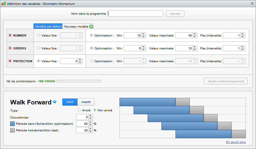
Research suggests using an optimization period representing 80% of the simulation period and 20% for the test period. It is also recommended that as many tests as possible be carried out to ensure the reliability of the analysis.
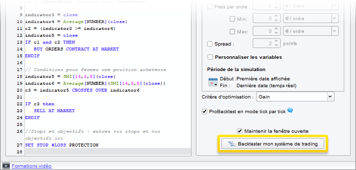
Once you’ve set your parameters, close the above window and launch the Walk Forward analysis by clicking on the “Backtest my trading system” button.
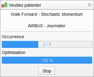
During Walk Forward analysis, the platform first optimizes the strategy over an initial period in the sample, and determines which set of variables generated the highest performance. Next, the performance of the same set of variables is tested on a separate sample.
The process is repeated 5 times. The aim is to determine whether the set of variables deemed optimal generates an in-line or even superior performance under different market conditions.
Depending on the number of variables and occurrences defined, calculations can be more or less complex.
Once calculations have been completed, a graphical representation of the profit & loss curve is displayed, together with a detailed report on system performance. In addition to the usual tabs, a new “Walk Forward Statistics” section presents a comparison of the different analysis periods for each repetition.
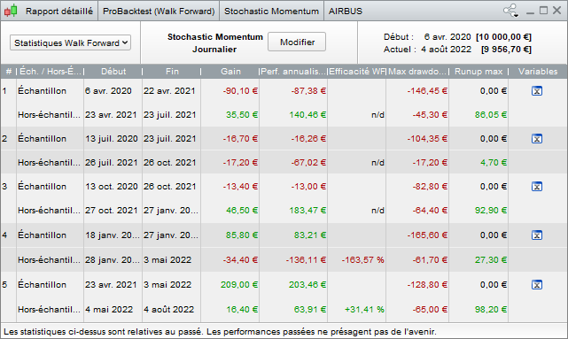
The platform aggregates and presents the results of the 1st optimization period (sample 1) and the 5 test periods (non-sample).
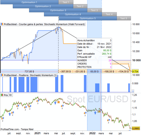
By placing the mouse cursor on the lower bands, the corresponding period is highlighted with the parameters used and the performance generated. In the screenshot above, the mouse is positioned on the 4th test period (non-sample period #4).
The best combination of PROTECTION, ORDERS and NUMBER variables from the 1st optimization phase (sample 4) was applied to the next test phase (highlighted). These parameters generated a gain of €2,250 over this period.
First and foremost, the strategy studied here appears to be robust. Only 2 out of 5 out-of-sample periods underperform in-sample periods. However, if the risk (represented by the Max drawdown indicator) measured during the test phases is in line with that measured during the optimization phases, the WFE ratios indicate the presence of a bias. A ratio that is too high may indicate over-optimization of the strategy or an abnormal market movement. If an economic event impacts too favorably on the strategy’s results, it is important to note that this impact could have been just as unfavorable if the markets had reacted differently to this exceptional event. It would therefore be interesting to carry out a larger number of occurrences and check whether this bias persists. If this is the case, the Walk-Forward analysis will have highlighted the risk of over-optimizing the strategy. The initial parameters should therefore be reviewed.
ProOrder – Automatic Trading
![]() Warning: If you set up a trading system using the ProOrder service, this service will automatically send signals, according to the parameters you have determined, for the execution of corresponding orders, without any individual validation of each order on your part being required. Your system will be executed automatically even when your computer is switched off. It is your responsibility to ensure that you have set up your system in such a way that it does not lead to losses in excess of an amount you are prepared to accept.
Warning: If you set up a trading system using the ProOrder service, this service will automatically send signals, according to the parameters you have determined, for the execution of corresponding orders, without any individual validation of each order on your part being required. Your system will be executed automatically even when your computer is switched off. It is your responsibility to ensure that you have set up your system in such a way that it does not lead to losses in excess of an amount you are prepared to accept.
In any event, ProRealTime will not be liable for any losses incurred as a result of your automatic trading system.
This part of the manual will explain how to go from backtesting your trading systems to running them as automated trading systems.
- The first section details how to send a trading system to ProOrder and the steps required to execute it in automatic trading.
- The second section shows how to launch an automatic trading system and check its performance.
- The third section describes the trading system parameters and their execution conditions.
- The fourth section explains how manual and automatic trading interact within the platform.
- The fifth section provides information specific to the execution of several automatic trading systems on the same instrument.
- The last section contains a list of indicators that cannot be used in automatic trading because of the way they are calculated.
We advise you to finish reading the manual before starting to run an automatic trading system.
Preparing a system for automatic trading execution
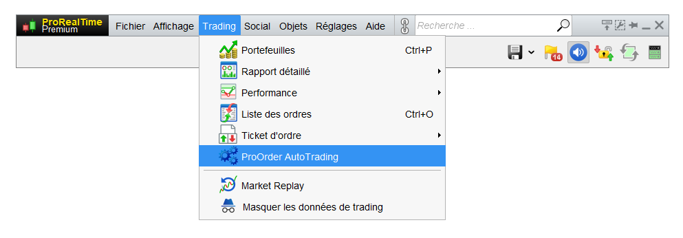
Start by opening the ProOrder window from the “Trading” menu:
The window shown below appears. It contains the steps to follow in order to prepare a system for automatic trading.
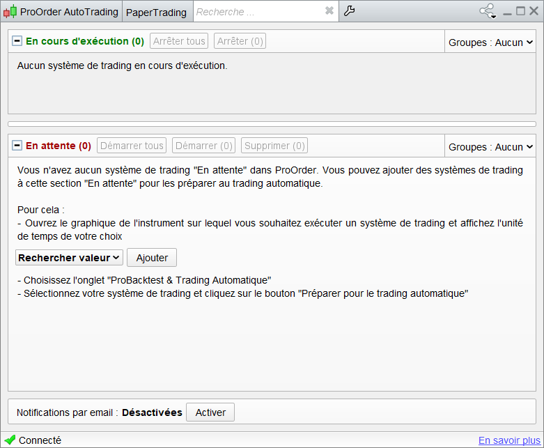
Choose a value and click on the “Add” button.
The “Indicators and Trading Systems” window appears. Click on the corresponding category to obtain a list of your automatic trading systems.
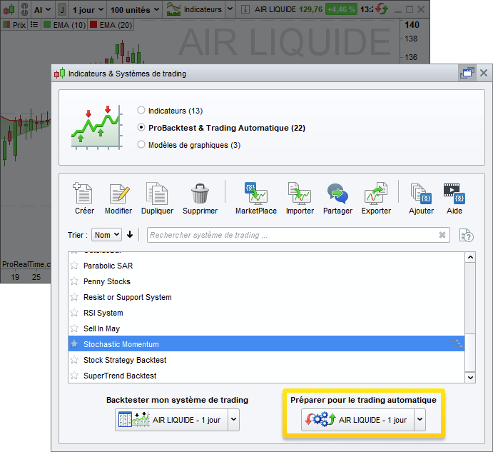
Select the system of your choice and click on “Prepare for automatic trading”. The system will then appear in ProOrder at the initially selected value.
Start a trading system with ProOrder and see how it performs
Once you’ve added a trading system to ProOrder, you can define its maximum position size parameter. Then launch your system by clicking on the “Start” button:
Be sure to read the confirmation pop-up: you will be asked to confirm the execution of the trading system. It’s important to understand that the maximum position size parameter takes precedence over the buy/sell quantities defined in the system code. The maximum position size for futures and Forex is defined in terms of number of contracts or number of lots. This lot size is defined by the broker and cannot be modified.
For example, if your code includes an instruction to buy 3 lots and the maximum position size limit is set to 1, the order to buy all 3 lots will be ignored.
Similarly, if your code successively calls for the purchase of 1 lot and then the short-sale of 3 lots, the short-sale order will be ignored and you will remain in a buy 1-lot position. We recommend that you always check the maximum position size parameter before launching a trading system.
For equities, the maximum position size is expressed as an amount (excluding brokerage fees).
Once launched, the system will be displayed in the “Running” section of the window, as shown below.
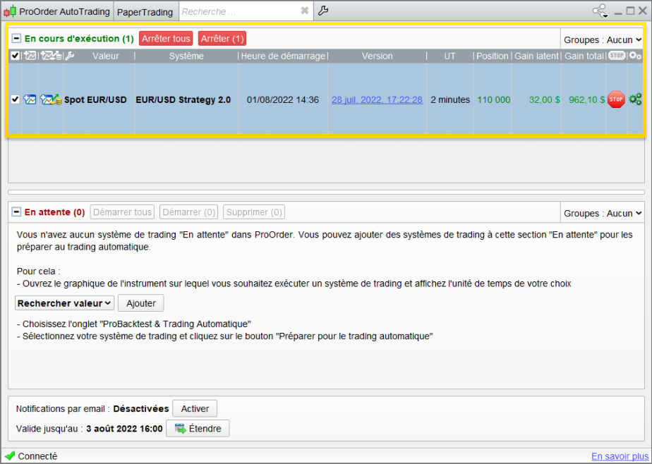
Once the system has been started, its positions, latent gains and total gains will be displayed in the ProOrder window. By clicking on the “Version” link, you’ll obtain a copy of the system code in question.
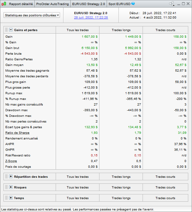
A detailed performance report and a system gain & loss curve can be obtained by using the corresponding button, as illustrated below.
Here’s an example of a gain & loss curve for a running system, with a detailed performance report:
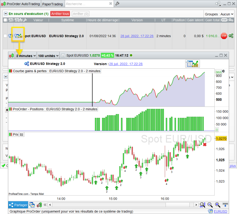
Note: The value of the gain displayed in the “Closed positions statistics” may differ from the value of the profit & loss curve. This is because the latter takes account of current open positions, which is not the case with the detailed report.
Automatic Trading parameters and execution conditions
Trading system parameters
It is advisable to configure your trading preferences before launching any automatic trading system. To do this, click on the wrench button as illustrated below:
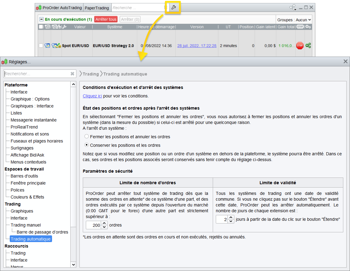
A link to the execution conditions of your trading systems is also available in this window. We strongly recommend reading this content to learn more about the behavior of your automatic trading systems.
Automatic shutdown of the trading system
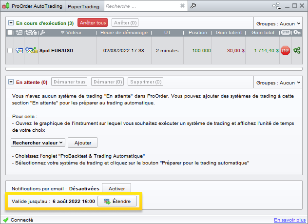
Validity date: All current trading systems have a common validity date. If you don’t click on the “Extend” button before this date, ProOrder may interrupt the corresponding trading systems. You can check the validity of your trading systems in the ProOrder window (the date displayed is based on your computer’s time zone). To extend the validity of your system, click on the “Extend” button at the bottom of the ProOrder window while a trading system is in progress.
The extension duration can be configured from the “Automatic Trading” tab of the “Trading Preferences” window. It is possible to change this duration even when systems are running: your changes will then be applied to the next extension.
Number of orders placed: ProOrder can interrupt a trading system if a maximum number of orders placed in a day is reached. You’ll find this setting in the “Automatic Trading” tab of the “Trading Preferences” window. If the number of pending orders cumulated with the number of open positions since the market opened (e.g. 00:00 GMT for Forex) exceeds the set parameter, the system will automatically stop. A pending order is an order sent to the broker which has not been executed, rejected or cancelled.
This corresponds, for example, to every “Stop“, “Trailing Stop” or “Target” instruction, as long as the associated order has not been executed, rejected or cancelled.
Also, 3 separate limit orders or 3 separate stop orders that have not been executed, rejected or cancelled will count as 3 pending orders (whether the 3 orders are at the same price level or not).
Take, for example, an automatic stop parameter set at 8 orders per day. Since the market opened, 5 orders have been executed by a given system. Currently, this system has 1 open position and 2 pending orders (a “Target” and a “Stop” order). The system now needs to send 1 additional order to the market: this 8th order will not be sent, as the stop level has been reached (5+2+1 = 8). As a result, the system will be interrupted, starting with the closing of pending orders, followed by the closing of active positions.
Order rejection: ProOrder can interrupt a trading system if too many of its orders have been rejected. The limit is fixed at 10 consecutive rejections.
Interaction between manual and automatic trading
When a trading system is running on a security, manual order placement is no longer available. However, manual trading remains possible on other instruments. A special button appears instead of the manual order bar on the instrument in question, as illustrated below:
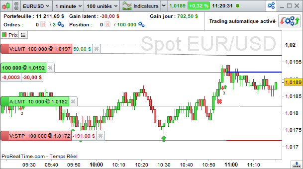
This button can be clicked to open the ProOrder window and view the status of trading systems currently running.
Launch several trading systems on the same instrument
NB: not applicable to all brokers.
If you run several trading systems on the same instrument, your overall net position is determined by all your systems. Let’s take an example where you have 2 trading systems. One places a buy order for 1 lot, while the other places a sell order for 1 lot. Your overall net position will then be 0. Only the overall net position is displayed if several systems are trading the same instrument.
When you display a system’s profit & loss curve, you also get its position histogram. Unlike the global net position, which aggregates all the data from the instrument’s systems, this histogram represents the positions taken by a single system. The position levels displayed may therefore differ, as illustrated in the graph below.
Example:
2 systems are running on the same instrument: one is in a sell position on 10 lots. The other is selling 6 lots. The net position is therefore equal to (10+6)= -16.

The net position of -16 also appears in the “Portfolios” window, available from the “Trading” > “Portfolios” menu:

When you run several trading systems on the same instrument, each system reports its own positions, orders, trades and profits independently. Consequently, LONGONMARKET or SHORTONMARKET instructions provide information on the Long or Short status of the system in question.
Your overall net position may differ from the position of a given system. The same applies to variables such as COUNTOFLONGSHARES, COUNTOFSHORTSHARES, COUNTOFPOSITION, POSITIONPRICE, STRATEGYPROFIT, TRADEINDEX, TRADEPRICE and POSITIONPERF, which only concern a given system.
Non-usable indicators
The following indicators cannot be used for automatic trading because their calculation method does not allow them to be used in real-time:
- ZigZag: signals based on this indicator are recalculated a posteriori. As a result, the signals given in real time can be very different from those given during backtesting.
- ZigZagPoint: signals based on this indicator are recalculated a posteriori. As a result, the signals given in real time can be very different from those given during backtesting.
- DPO
Note on Customized Time Zones and Market Hours
When a trading system is sent to the ProOrder module, the strategy will be associated with the customized time zone and market hours defined on the market to which the instrument belongs. These settings will be applied each time the strategy is launched. To change a strategy’s time zone or custom market hours, it is necessary to remove the strategy from ProOrder, modify these settings in the “Options/Intraday chart time zones and ranges” menu and return the strategy to ProOrder.
Please refer to the Customize Time Ranges section for instructions relating to the chart’s time zone and the operation of customized market hours.
- Introduction
- Programming trading systems
- Programming with ProBuilder
- Stops and Targets
- Protective stops
- Follower stops
- Using "Set Target / Set Stop" with an "IF" conditional instruction
- Multi-level stops and limits
- Stop a trading system with QUIT
- Position monitoring
- State variables
- Position size variables
- LongTriggered
- ShortTriggered
- TradeIndex
- TradePrice
- PositionPerf
- PositionPrice
- StrategyProfit
- Definition of execution parameters for trading systems
- Cumulative orders in the same direction
- Preload history
- FLATBEFORE and FLATAFTER
- Reinvest gains (backtests only)
- MinOrder and MaxOrder (backtests only)
- Calling up indicators
- Programming tips
- ProBacktest - Trading system simulation
- Capital / Money Management
- Variable optimization
- Setting the backtest execution period
- Customize time slots for backtests
- Reasons for stopping a ProBacktest
- Displaying backtest variable values
- The Walk Forward method
- ProOrder - Automatic Trading
- Preparing a system for automatic trading execution
- Start a trading system with ProOrder and see how it performs
- Automatic Trading parameters and execution conditions
- Interaction between manual and automatic trading
- Launch several trading systems on the same instrument
- Non-usable indicators
- Note on Customized Time Zones and Market Hours